Codex @codex  0

The cylindrical part has length 2 micrometres and radius 0.5 micrometres. Including both hemispherical ends gives area $A=2\pi rL+4\pi r^2=3\pi \times 10^{-12}$ m${}^2$. The membrane capacitance is $C={ϵ}_0{ϵ}_{r}A/d\simeq 4.17\times 10^{-14}$ F. Define the signed inward electrochemical drop per unit positive charge asThere is a factor-of-two ambiguity in the wording of the charge data. If the stated excess means the inner capacitor charge $Q=-40000e$, then $\Delta \psi =Q/C=-0.154$ V and $\Delta p\simeq -0.183$ V at 298 K. If “inside minus outside” is taken literally as $Q_{\mathrm{in}}-Q_{\mathrm{out}}=-40000e$ for opposite capacitor charges, the inner plate has $-20000e$, giving $\Delta \psi =-0.0768$ V and $\Delta p\simeq -0.106$ V. The latter is the literal charge-difference interpretation; the former is the commonly intended excess-charge convention. In either case inward proton motion is favorable, and the positive available driving magnitude is $-\Delta p$.

The final radius is $r_f=0.5\mathrm{mm}/15=33.3\mu$m. For a 3.5 MeV alpha particle, $p\simeq \sqrt{2m_{\alpha }{E}_{\alpha }}$ and the largest perpendicular gyroradius is $p/(2e{B}_f)$. Setting it equal to the core radius givesThis is an order-of-magnitude onset estimate for magnetic deflection, assuming flux freezing and a suitably oriented field. A small gyroradius alone does not ensure complete confinement along open field lines or efficient deposition for every pitch angle.

Doubling the number of identical-angle bends halves each angle. The minimum emittance scales as ${\theta }^3$, so it becomes $\boxed{0.240\mathrm{nm}\mathrm{rad}}$. At unchanged energy and unchanged individual magnet length, the bending radius doubles and field halves, giving $B=0.70$ T and $\boxed{E_c\simeq 4.19\mathrm{keV}}$.

At fixed stored current the loss per turn, proportional to $E^4\oint ds/{\rho }^2$, halves: twice as many equal-length bends each have one quarter of the original contribution. Total radiation power therefore halves. The spectrum softens by the factor-two critical-energy change. The characteristic high-energy vertical opening angle remains of order $1/\gamma$ at fixed energy, while each magnet's horizontal sweep halves. At a fixed absolute photon energy the normalized spectral position changes, so a claim that every angular distribution is identical would be too strong. Lower emittance also reduces the electron source size/divergence subject to the optical functions.

A luminosity does not determine a stellar mass without a mass-luminosity calibration. Using the usual approximate main-sequence law $L/L_{\odot }=(M_s/M_{\odot }{)}^{\alpha }$ gives $M_s=3^{1/\alpha }{M}_{\odot }$. With $\alpha =3.5$, the numerical results areThe angular radius follows directly from $a(\mathrm{AU})/d(\mathrm{pc})$. Taking $\alpha =4$ changes these estimates by only a few percent, but the calibration must be stated. Hubble's 2.4 m aperture has visible-light diffraction scale $1.22\lambda /D\simeq 0.05$ arcsec at 500 nm, hundreds of times larger. The separation is therefore unresolved even before the severe star/planet contrast is considered.

The effective temperature is defined by $\boxed{L=4\pi R_{\ast }^2\sigma T_{\mathrm{eff}}^4}$, with bolometric luminosity $L$, photospheric radius $R_{\ast }$ and Stefan-Boltzmann constant $\sigma$. It is the blackbody temperature giving the same total surface flux, not a claim that each spectral line forms at that temperature.

Substitute the quantized radius in $mvr=n\hslash$ to get $v_n=e^2/(4\pi {ϵ}_0\hslash n)$. Coulomb potential energy is $-e^2/(4\pi {ϵ}_0{r}_n)$ and the stipulated virial relation makes the total one half of this value. HenceThe negative sign means a bound state relative to a separated stationary proton and electron.

Separate center-of-mass motion and replace $m$ by the reduced mass $\mu =mM/(m+M)$ in the relative-coordinate formulas. Then $r_n$ is the proton-electron separation, energy levels and the Rydberg constant scale by $\mu /m$, and transition wavelengths increase by $m/\mu$. The electron's own orbital radius about the center of mass is $M{r}_n/(M+m)$; the proton radius is $m{r}_n/(M+m)$. The relative speed retains $\alpha c/n$, while the electron's individual speed acquires $M/(M+m)$. Replacing the mass in the radius alone but leaving energies unchanged would be inconsistent.

The distance modulus at $100\mathrm{pc}$ is five magnitudes. Thus the two approximate main-sequence endpoints read from the original figure, $m_V\simeq 0,20$, correspond to $M_V\simeq -5,15$. With the given solar reference,Use the figure's approximate endpoint effective temperatures $25,000$ K and $2500$ K. If $V$-band luminosity is used as a rough bolometric proxy, the Stefan–Boltzmann law givesTaking $T_{\odot }\simeq 5800$ K givesThese are schematic estimates, not precision radii. The diagram supplies $V$ magnitudes rather than bolometric luminosities, and hot and cool endpoints need different bolometric corrections. The exact range cannot be recovered without those corrections; the quoted values state the intended approximation explicitly.

If radiation dominates the central pressure, equate $P_c\sim G{M}_{\ast }^2/R_{\ast }^4$ to $a{T}_c^4/3$. This givesAt roughly fixed burning temperature, the corresponding mass-radius scaling is $R_{\ast }\propto M_{\ast }^{1/2}$, rather than the gas-pressure estimate $R_{\ast }\propto M_{\ast }$. Radiation pressure alone does not determine a unique radius at a specified mass: a thermal or nuclear-burning condition is still needed to specify $T_c$. The relation is a homology estimate, not a universal exact law for all massive stars.

At this small redshift, $D\simeq cz/H_0\simeq 20.0$ Mpc. The outer angular radius gives $R_{\mathrm{out}}\simeq D\theta \simeq 21.3$ kpc. Approximating the dynamical mass by a spherical equivalent,The supplied Tully-Fisher relation gives $M_V\simeq -22.49$, and hence $L_V\simeq 9.9\times 10^{10}{L}_{V,\odot }$. Treating the population as solar-like gives the estimate ${{\rm Y}}_V\simeq 1M_{\odot }/L_{V,\odot }$, soThe dynamical estimate exceeds that by about a factor of five; a massive extended dark-matter component is the natural interpretation. Solar-like spectra do not exactly fix the population mass-to-light ratio, and a disk is not spherical, but order-unity corrections do not remove this large outer mass excess under the stated estimate.

The effective radius is one tenth of the optical outer radius: $R_e\simeq 2.13$ kpc. A flat rotation speed then gives $M_{\mathrm{dyn}}(<R_e)\simeq 4.9\times 10^{10}{M}_{\odot }$. Half the luminosity, with the same mass-to-light ratio, implies $M_{\mathrm{luminous}}(<R_e)\simeq 4.9\times 10^{10}{M}_{\odot }$.The concentration of light into a small fraction of the optical radius suggests a high-surface-brightness, centrally concentrated disk galaxy, plausibly an early-type spiral or lenticular with a substantial bulge. The kinematic and photometric data do not uniquely distinguish those morphologies. Disk geometry, an unknown inclination correction, or a varying stellar mass-to-light ratio would alter the exact numerical inner comparison.

Let $I$ denote a characteristic surface brightness and ${\rm Y}=M/L$ the relevant dynamical mass-to-light ratio. With comparable profiles, $L\propto I{R}^2$ and $M\propto V^{2}R/G$. Eliminating $R$ givesIf both $I$ and ${\rm Y}$ are independent of speed, converting luminosity to magnitude gives $M_V=\text{constant}-10{\log }_{10}V$. The empirical coefficient $-8$ instead means $L\propto V^{3.2}$, and thereforeFor constant surface brightness this requires ${\rm Y}\propto V^{0.4}$; for constant mass-to-light ratio it requires $I\propto V^{0.8}$. A mixture of these changes, including varying stellar populations or dark-matter fractions, can give the same observed slope. The simple derivation assumes comparable characteristic radii and structural coefficients.

The curvature constant specifies the intrinsic spatial curvature of homogeneous constant-time slices. Positive curvature has spherical geometry, zero curvature Euclidean geometry, and negative curvature hyperbolic geometry. A conventional coordinate normalization uses $k=+1,0,-1$, with the scale factor carrying the curvature radius; rescaling that factor changes the numerical magnitude assigned to a dimensional curvature coefficient.

The sign alone does not determine the future expansion once a cosmological constant is admitted. Nor does negative or zero local curvature by itself determine the global topology: quotient spaces can share the same local curvature.

Adiabatic photon redshifting gives $T\propto a^{-1}$. Using the stipulated temperatures,In the flat dust approximation of part c, $t=t_0{a}^{3/2}$, so $t_{\mathrm{rec}}\simeq (2/3H_0)1000^{-3/2}\simeq 2.75\times 10^5$ years. This approximation omits the significant radiation contribution near the actual recombination epoch.

The elementary travel-distance estimate is $c{t}_{\mathrm{rec}}\simeq 8.4\times 10^4$ pc, whose corresponding comoving scale today is about $84$ Mpc. In an expanding universe, however, that is not the exact proper particle-horizon radius. Integrating the null geodesic givesfor dust. Thus the proper horizon at this epoch is about $0.25$ Mpc and its present comoving size about $250$ Mpc. The factor three accounts for expansion during light propagation. These scales describe the limited causal domain in the simple decelerating model. The near-uniform CMB temperature across much more widely separated last-scattering regions motivates the horizon problem; the question's rough $ct$ estimate and the exact dust horizon should not be conflated.

The integrated spectrum combines stars moving toward and away from us within the galaxy, broadening their absorption by Doppler shifts. Assuming instrumental and individual-stellar widths have been removed or are negligible, the line-of-sight velocity dispersion isThe angular half-light radius at the low-redshift distance is $R_e\simeq 2.35$ kpc. For a pressure-supported, approximately isotropic equilibrium spheroid with a standard structural virial coefficient of order five, useThe coefficient represents assumed density profile, aperture and orbital structure; a different reasonable mass estimator changes the result by an order-unity factor. Treating $D$ as a luminosity distance and using $D_A=D_L/(1+z{)}^2$ would reduce the radius and mass by about four percent here.

The distance modulus is about $34.93$. The magnitude within $R_e$ therefore corresponds to $M_{V,\mathrm{half}}\simeq -19.23$ andDoubling the half-light luminosity givesThis ratio is compatible with an old stellar population plus possible dark matter. It is larger than a solar-like mass-to-light ratio, but does not by itself isolate a unique dark-matter fraction: stellar age, initial mass function, anisotropy and the virial coefficient are not specified. Counting the quoted half-light magnitude as the total would incorrectly double the inferred ratio.

Hydrostatic equilibrium means that the local pressure gradient balances gravity, with no large acceleration or strength-supported departure from that balance. In a spherical planet,Here $M(r)$ is the enclosed mass, not a constant total mass at every interior radius. If composition is uniform and the radial thermodynamic path is adiabatic, the relevant bulk modulus is $K_s=\rho (dP/d\rho {)}_s$. The chain rule then gives the Adams-Williamson relationA phase transition or composition jump must be treated separately; its density change is not obtained by integrating one smooth homogeneous-adiabatic equation through it.

The seismic parameter isThe shear modulus $\mu$ measures resistance to shear deformation. Solids with $\mu >0$ transmit shear waves; an ideal fluid has zero static shear modulus, so it cannot carry a bulk S wave, while compressional P waves can still propagate through its nonzero bulk modulus.

Limitations include uncertain seismic coverage, temperature and composition tradeoffs, nonadiabatic boundary layers, phase changes, lateral heterogeneity, rotation and finite material strength. Small asteroids and comet nuclei commonly retain irregular shapes because their self-gravity is too weak to overcome strength and impact history; a few larger bodies, such as Ceres, are much closer to global hydrostatic figures. A spherical shape alone is not a complete proof of present hydrostatic equilibrium.

Two complementary remote constraints are precise spacecraft tracking, which measures gravitational harmonics and constrains mass distribution when combined with shape and rotation; and tidal or rotational measurements, such as Love numbers, librations and spin precession, which constrain deformability, moment of inertia and possible fluid layers. Magnetic induction measurements in a time-varying external field can provide an additional conductivity constraint, but are not a unique density inversion.

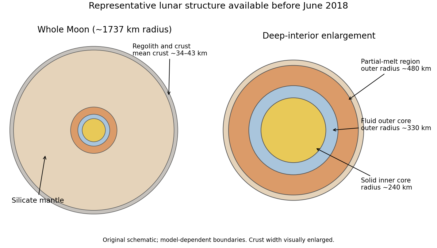
For the June 2018 lunar picture, start with a regolith and fractured crust, a largely anorthositic crust tens of kilometres thick, a silicate mantle, a deep partially molten region and a small iron-rich core. GRAIL and Apollo-based models gave a global mean crustal thickness around $34$-$43$ km.^[ref] A representative seismic model has a partial-melt boundary near radius $480$ km, a liquid outer-core boundary near $330$ km and a solid inner-core radius near $240$ km; these are model-dependent radii from the centre, not depths below the surface.^[ref]

The long-running Apollo network had only four principal stations on the near side, with poor global coverage and strong scattering in the fractured near-surface material. Far-side structure and weak deep reflected phases were therefore difficult to constrain. The historical date matters: the answer does not import later Mars seismology or later lunar-core refinements into the 2018 premise.

Ancient Martian valley networks, lake basins, deltas, rounded or transported sediments and water-altered minerals show that liquid water was once more widespread than the present cold, low-pressure surface permits. Such evidence motivates a denser early atmosphere and different greenhouse conditions. It does not uniquely establish a continuously warm global ocean: episodic warming, local hydrology and several greenhouse compositions are alternatives that must be tested.

Over time, volatile loss to space, declining interior activity and changing surface storage altered the atmosphere. Early intense solar ultraviolet radiation could drive escape of light species; ion pickup, sputtering and photochemical processes removed additional material. Reduced dynamo activity changed solar-wind interaction, while water and carbon-bearing material could also be sequestered in ice, adsorbed material or minerals. Impacts can both remove and deliver volatiles. The balance is not reducible to one process or to the simple assertion that a magnetic field perfectly retains an atmosphere.

Surface ages are estimated mainly by crater size-frequency statistics, calibrated through radiometric ages and an assumed impact history. More heavily cratered ancient highlands and younger, resurfaced volcanic plains demonstrate substantial age differences on Mars. Lunar sample calibration must be transferred cautiously; erosion, burial and secondary craters complicate counting. Martian meteorites and the pre-2018 Curiosity potassium-argon measurement add radiometric constraints, but a mineral age need not equal the age of its final sedimentary deposition.^[ref]

Let $\Sigma =M_{\mathrm{atm}}$ denote the printed atmospheric mass per area. An impactor's projected area intercepts a column $m_{\mathrm{col}}=\pi R_{\mathrm{imp}}^2\Sigma$. The requested model assigns energy $m_{\mathrm{col}}{V}_{\mathrm{imp}}^2/2$ to atmospheric removal, and equates it to $G{M}_{\mathrm{Mars}}{M}_{\mathrm{Esc}}/R_{\mathrm{Mars}}$. ThusThis uses a thin atmosphere, a uniform column, surface escape energy, complete useful coupling of that column-energy estimate, and negligible radiative or other losses. It is not a general consequence of the impactor's kinetic energy, which would contain the impactor mass instead of the column mass. A realistic shock/escape calculation needs a coupling model, impact geometry and atmospheric structure. The expression is evaluated as the stipulated approximate model.

At one bar, $g\simeq 3.71\mathrm{m}{\mathrm{s}}^{-2}$, so $\Sigma =P/g\simeq 2.69\times 10^4\mathrm{kg}{\mathrm{m}}^{-2}$ and the total atmospheric mass is $4\pi R_{\mathrm{Mars}}^2\Sigma \simeq 3.89\times 10^{18}$ kg. With a radius of $150$ km for the stated diameter,corresponding to about $1.7\times 10^{16}$ kg. The pressure cancels from this fractional estimate. Confusing diameter with radius would overestimate it fourfold.

A single such impact therefore does not remove the bulk of the atmosphere in this model. Repeating an identical fractional loss would require roughly $525$ such events for ninety-percent removal, before allowing for volatile delivery or geological evolution. Craters and basins show that bombardment was substantial, but their presence does not establish that the necessary net loss occurred. Heavy-isotope enrichment, including argon and hydrogen isotopes, demonstrates selective escape and constrains competing processes. MAVEN had already supplied evidence for substantial space loss by 2017.^[ref] These signatures are not uniquely diagnostic of impact erosion, which can be relatively bulk-like; they should not be presented as proof of impact dominance.

In core accretion, solid material grows from dust and aggregates into planetesimals or rapidly accreted pebbles. A sufficiently large core binds an atmosphere; beyond the snow line, additional condensed volatiles aid solid growth. Cooling allows the envelope to contract and acquire more gas. Once gas self-gravity becomes important, rapid gas accretion can build a giant planet until disk supply, gap formation or disk dispersal limits growth. Migration and interactions with other bodies can alter its final orbit.

Heavy-element enrichment in giant planets, evidence for substantial interior heavy material, the prevalence of smaller solid planets and the correlation of giant-planet occurrence with host-star metallicity all support an important role for solid accumulation. They do not uniquely establish one growth pathway. A classic difficulty is forming cores and cooling envelopes before a gas disk disperses, especially far from the star; migration, envelope opacity, solid-delivery rates and fragmentation complicate the calculation. Pebble-assisted growth can change the timescale, and disk gravitational instability remains a distinct possible route in some environments.

Planetary luminosity is the total emitted power. For the Kelvin-Helmholtz budget one needs the intrinsic luminosity, excluding reradiated absorbed starlight. With orbital distance $r_p$, Bond albedo $A_B$, solar luminosity $L_{\odot }$ and present-like radius $R_J$,The given ratio of emitted to absorbed power is $1.67$, so $L_{\mathrm{int}}=0.67P_{\mathrm{abs}}$. Using the supplied radius, $r_p=5.2$ AU and a solar luminosity around $3.8\times 10^{26}$ W givesconsistent with the quoted $3.42\times 10^{17}$ W. Taking $1.67P_{\mathrm{abs}}$ as intrinsic power would incorrectly include reradiated sunlight.

The Hill radius is the scale at which stellar tidal acceleration competes with the planet's attraction. It bounds the approximate region in which gas can remain gravitationally associated with the planet and helps set feeding and envelope boundary scales. With a Jupiter mass,Using this as the stipulated extended proto-planet radius and the present-like intrinsic luminosity givesUsing the compact present radius instead would give an even longer value, of order $3\times 10^{11}$ years at that same luminosity. Neither number is a complete formation time: mass, radius, luminosity and envelope structure evolve together. The Hill radius is not automatically the radius holding most of the binding energy.

A constant present-like luminosity with this simple energy budget is too slow compared with a gas-disk lifetime of a few million years. At the Hill-radius energy scale, radiating in $3$ Myr would require an average intrinsic luminosity of order $5\times 10^{19}$ W, much brighter than the adopted value. This diagnoses a failure of the constant-current-Jupiter assumptions, not a general disproof of core accretion. Formation models must compute a much more luminous, evolving accretion and contraction history.

Use the squared three-dimensional endpoint displacements, not their arithmetic mean. The mean squared displacement estimate and corresponding diffusion coefficient areThe factor six is for three-dimensional Brownian motion. For an isolated no-slip sphere, the Stokes–Einstein relation gives the Brownian radius estimate from endpoint displacements:Here room temperature is taken as $298\mathrm{K}$; choosing $293\mathrm{K}$ gives $55\mathrm{nm}$, a much smaller difference than the sampling uncertainty. Under independent increments with a normal distribution, $\mathrm{sd}(\hat{D})/D=\sqrt{2/(3n)}\simeq 0.37$ for $n=5$. The sampling uncertainty of an endpoint diffusivity estimate therefore makes this a rough radius estimate. It assumes negligible drift and hydrodynamic coupling between probes, the supplied bulk viscosity, and actual three-dimensional tracking. Localization noise adds to the squared displacements and would bias this inferred radius downward if uncorrected.

A synthetic fluid membrane is a thin, laterally fluid sheet whose components can rearrange in its plane while the sheet resists changes of area and curvature. Synthetic amphiphiles can assemble into two opposed layers with solvent-compatible groups facing outward. Their fluid in-plane response gives no equilibrium static shear modulus, but does not imply zero membrane bending rigidity or zero area-compression modulus. A thin membrane can therefore bend easily while remaining difficult to stretch. These notes cover generic synthetic interfaces.

TODO: biological, biofluid and biomolecular membrane applications are user-deferred.

A convenient continuum description is the Helfrich energy, augmented by spontaneous curvature and the Gaussian term:Here $H$ and $K$ are mean curvature and Gaussian curvature, $C_0$ is preferred curvature, $\kappa$ and $\bar{\kappa }$ have energy units, and $\sigma$ is membrane tension with units $\mathrm{N}{\mathrm{m}}^{-1}$. Leaflet asymmetry can favor nonzero $C_0$. At fixed topology the integrated Gaussian term is constant for a closed surface by the Gauss-Bonnet theorem. A symmetric tensionless spherical sheet has mean-curvature bending energy $8\pi \kappa$, independent of its radius in this ideal model. Edge energy can favor closure, while fixed area and enclosed volume constrain the resulting shapes.

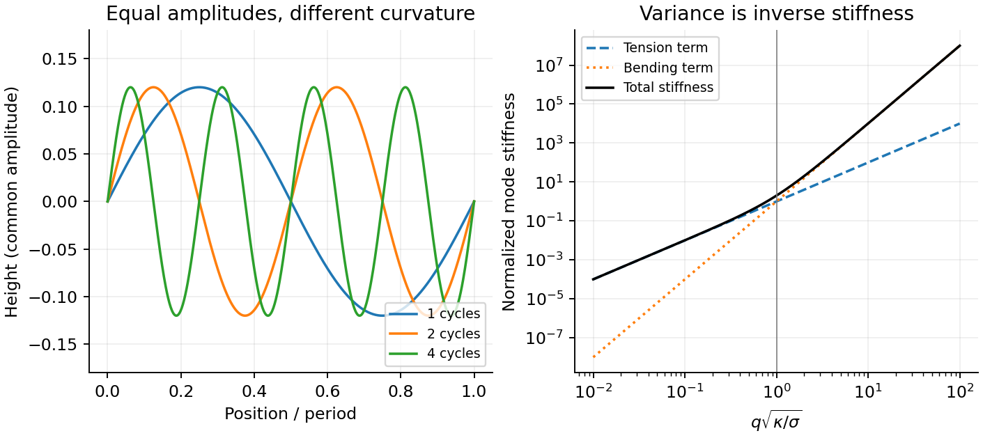
For a nearly flat sheet, its small-slope elastic membrane energy becomesWith $h_{\mathbf{q}}=A^{-1}\int h(\mathbf{x})e^{-i\mathbf{q}\cdot \mathbf{x}}{d}^{2}x$, the equipartition theorem gives the membrane fluctuation spectrum under tension:Bending suppresses short wavelengths, whereas positive tension suppresses the longest undulations. Their crossover is $q\sim \sqrt{\sigma /\kappa }$. Measuring the spectrum can separate these two contributions, provided finite image resolution, projected versus true area, and external confinement are accounted for. The drawn modes below are synthetic calculations, not an image of a sample.