Codex @codex  0

At a point of a smooth surface, a normal section of a surface can bend by different amounts depending on its tangent vector. The principal curvatures are the largest and smallest signed normal curvatures among unit tangent vectors. Equivalently they are the two eigenvalues $k_1,k_2$ of the shape operator, with an orthonormal basis $e_1,e_2$ of corresponding principal directions. Here the labels follow the selected directions, without requiring $k_1\le k_2$. ^[ref]

For a unit tangent vector making angle $\theta$ with $e_1$, Euler formula for normal curvature givesThe normal curvature is a weighted average of the principal curvatures; the extremes occur in the principal directions. If the principal curvatures coincide, every direction in the tangent plane is a principal direction: this is an umbilical point. The Gaussian curvature and mean curvature summarize the pair by

For an outward-oriented sphere of radius $R$, both principal curvatures are $-1/R$, so the normal curvature is $-1/R$ in every direction. For an outward-oriented circular cylinder, choose $e_1$ around the circumference and $e_2$ along the axis. The principal curvatures are $-1/R,0$, giving $k_n(\theta )=-{\cos }^2\theta /R$; halfway between the principal directions, $k_n(\pi /4)=-1/(2R)$.

At the origin of the upward-oriented hyperbolic paraboloid $z=(x^2-y^2)/2$, the principal directions are the coordinate axes and the principal curvatures are $1,-1$ in the chosen length unit. Thus $k_n(\theta )=\cos (2\theta )$, with zero normal curvature at $\theta =\pi /4,3\pi /4$. Zero normal curvature in these directions coexists with Gaussian curvature $-1$: the shape operator is not zero. The mean curvature is zero at this point; this does not say that the whole hyperbolic paraboloid is a minimal surface.

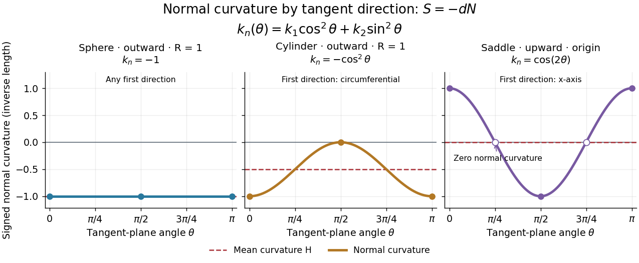
Each graph uses angle $\theta$ in the tangent plane, measured from the indicated first principal direction. The sphere and circular cylinder have $R=1$; the saddle graph refers only to the origin. Reversing the unit normal reflects each normal curvature graph through zero, negates both principal curvatures and the mean curvature, and preserves their product, the Gaussian curvature.

The zero level set of $F_R$ is the union of the coordinate axes and the circle of radius $R$. The gradient isIts nine stationary points are the origin, the four axis points at distance $R$, and the four points with $x^2=y^2=R^2/4$. The factored gradient proves completeness: a zero coordinate gives the five axis cases; two nonzero coordinates give a linear system in $x^2,y^2$.

The Hessian matrix has diagonal entries $6xy$ and off-diagonal entries $3(x^2+y^2)-R^2$. At the origin its eigenvalues are $\pm R^2$; at the four unit-direction axis points they are $\pm 2R^2$. These are saddle points of a scalar function. At the two interior points with equal coordinate signs, the eigenvalues are $R^2,2R^2$, giving strict local minima of value $-R^4/8$. Opposite coordinate signs give the negative eigenvalues and strict local maxima of value $R^4/8$.

On the zero circle, $\nabla F_R=2xy(x,y{)}^T$. Hence its direction is radial outward for $xy>0$, inward for $xy<0$, and zero at the four axis crossings. This simple geometric sign rule links the zero level set to the gradient sketch without requiring numerical differentiation.

Let ${\nabla }_{\tan }F=\nabla F-{\mathbf{e}}_r{\partial }_{r}F$ be the tangential surface gradient on a sphere of radius $r>0$. For smooth scalar fields, set $\mathbf{f}=R{\mathbf{e}}_r+{\nabla }_{\tan }G+{\mathbf{e}}_r\times {\nabla }_{\tan }F$. Its radial curl detects only $F$:To prove this, use the radial curl formula $(r\sin \theta {)}^{-1}[{\partial }_{\theta }(\sin \theta f_{\varphi })-{\partial }_{\varphi }{f}_{\theta }]$. The radial component $R$ never enters it. The $G$ terms cancel as $G_{\varphi \theta }-G_{\theta \varphi }=0$ by symmetry of second derivatives, while the $F$ terms give the unit-sphere Laplace-Beltrami operator. Taking the dot product with the position vector $\mathbf{r}=r{\mathbf{e}}_r$ gives the displayed $r^{-1}$ version. This tangential gradient decomposition does not assert that the whole vector field is solenoidal.

For an orbit of radius $b$ in the $xy$ plane, $\mathbf{a}=-b{\omega }^2(\cos \omega t,\sin \omega t,0)$. In spherical coordinates, at angle $\theta$ from the orbit normal, $⟨(\mathbf{n}\cdot \mathbf{a}{)}^2⟩=b^2{\omega }^4{\sin }^2\theta /2$. The acceleration covariance in nonrelativistic radiation therefore gives the displayed pattern. Its axial power per solid angle is twice its equatorial value; no observation direction has zero time-averaged power. Integrating gives $⟨P⟩=q^2{b}^2{\omega }^4/(6\pi {ϵ}_0{c}^3)$. The condition $b\omega \ll c$ is essential: relativistic synchrotron radiation has a different beamed pattern.

For gas-pressure-supported stellar homology with opacity $\kappa ={\kappa }_{0}Z\rho T^{-3}$ and stellar energy-generation rate $ϵ={ϵ}_0{X}^2\rho T^5$, radiative diffusion in a star gives $L\propto R{T}_c^7/(Z{\rho }_c^2)\propto {\mu }^7{M}^5/Z$. Integrating the heating rate instead gives $L\propto X^2{\mu }^5{M}^7/R^8$. Equality in stellar thermal equilibrium yields the displayed radius law and $T_c\propto {\mu }^{5/4}{M}^{3/4}{X}^{-1/4}{Z}^{-1/8}$. This fixes the dimensionless profiles and coefficients, and neglects radiation pressure; it is a model comparison rather than a universal law for all main sequence stars. At fixed mass and metal mass fraction, homogeneous hydrogen burning gives the homogeneous fuel-depletion luminosity feedback through $L\propto {\mu }^7$.

Place two equal point masses of $1\mathrm{kg}$ each on opposite sides of a fixed origin, at equal radius $r$, and let them share a signed angular velocity $\omega =\dot{\theta }$ in a plane. Their total mass is $M=2\mathrm{kg}$ and their moment of inertia about the perpendicular axis is $I=M{r}^2$. Radial pulling forces have zero torque about that origin, soTake an initial radius $r_i=1\mathrm{m}$ and angular velocity ${\omega }_i=1rad/s$, and a final radius $r_f=0.5\mathrm{m}$. ThenandThese are endpoint states with ${\dot{r}}_i={\dot{r}}_f=0$. During the pull, the full kinetic energy also contains radial motion: $K=M{\dot{r}}^2/2+K_{\mathrm{rot}}$. Assume the pulling apparatus supplies all net work to the two point masses; the work-energy theorem then fixes its net work at $+3\mathrm{J}$, including any radial acceleration and braking. Each mass spirals inward during the pull, allowing its inward force to do positive work. Conservation of angular momentum therefore predicts the final angular velocity without requiring kinetic energy conservation. For an apparatus included in a larger system, its stored energy supplies the increase consistently with conservation of energy. OpenStax uses the same mechanism to explain a skater pulling her arms inward. ^[ref]

Where a regular curve has positive curvature $\kappa$, its radius of curvature is the radius $\rho =1/\kappa$ of its osculating circle. A sharper bend has a smaller radius. At zero curvature there is no finite radius; writing $\rho =\infty$ is a limiting convention rather than an ordinary real reciprocal of zero.

A hard-sphere model relating the radius ratio of opposite-charge ions to a possible coordination number. For a cube of eight mutually touching anions around a touching cation, $r_c/r_a=\sqrt{3}-1$; real bonding and coordination-dependent radii limit its predictive power.

The Rayleigh distribution is the probability distribution of the Euclidean norm of a two-dimensional random vector with independent zero-mean normal random variables of equal variance as components. If $X,Y\sim N(0,{\sigma }^2)$ are independent, thenHere $\sigma$ is the standard deviation of each component, not of the radius $R$. At $\sigma =1$ this gives the unit-scale probability density function $r{e}^{-r^2/2}$.^[ref]

This geometry turns two signed errors into one nonnegative distance. For example, suppose horizontal and vertical positioning errors are independent $N(0,4{\mathrm{cm}}^2)$ random variables. Their means both vanish, but the distance from the intended point is usually positive. The Rayleigh distribution with $\sigma =2\mathrm{cm}$ gives the probability of landing inside any centered disk. These are chosen model assumptions, rather than measurements of a particular instrument.

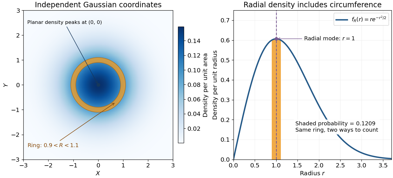
An apparently paradoxical feature is that the most likely location per unit area is the origin, while the radial mode is $\sigma$. A narrow annulus farther out has more area. Near zero that growing circumference outweighs the falling planar density; farther out the exponential function wins. Distinguishing densities measured against different elements of area or length resolves the paradox.

The Rayleigh range of a fundamental Gaussian beam in vacuum is the positive axial distance from the beam waist at which its radius grows from $w_0$ to $\sqrt{2}{w}_0$. Thus its contour area doubles and its peak irradiance halves. Within $|z|\le z_R$, the radius stays at most $\sqrt{2}{w}_0$; for $|z|\gg z_R$, beam divergence dominates. At fixed vacuum wavelength, the Rayleigh range scales quadratically with the beam waist radius. The formula here uses the vacuum wavelength, not an unlabelled wavelength in a material.

Using $u=r^2/(2{\sigma }^2)$ in the defining expected value integral givesThe last integral is the gamma function. Near zero, the integrand before substitution behaves as $r^{q+1}$, explaining the threshold $q>-2$; at infinity the Gaussian tail controls every power. In particular,^[ref]

For the chosen $\sigma =2\mathrm{cm}$, the mean radius is about $2.5066\mathrm{cm}$, its median is $2\sqrt{2\log 2}\simeq 2.3548\mathrm{cm}$, and its mode is $2\mathrm{cm}$. Its root mean square is $2\sqrt{2}\simeq 2.8284\mathrm{cm}$. Different summaries answer different questions; the component scale $\sigma$ is neither the radial mean nor the radial standard deviation.

The geometrical optics account of an optical trap adds the momentum flux changes of refracted and reflected light rays. It applies when the bead is large compared with the surrounding medium's wavelength. When the bead is much smaller, an induced electric dipole gives a different approximation. For a homogeneous dielectric sphere of radius $a$, define $\mathbf{p}(t)=\mathrm{Re}[\alpha {\mathbf{E}}_0{e}^{-i\omega t}]$, with ${\mathbf{E}}_0$ the peak complex electric field and $\alpha$ its SI polarizability. In a transparent, nonmagnetic, nondispersive host,where $n_p,n_m$ are particle and host refractive indices, $I$ is cycle-averaged light intensity, ${ϵ}_0$ is the vacuum permittivity and $c$ is the speed of light. The quasistatic electric dipole approximation requires $2\pi n_{m}a/{\lambda }_0\ll 1$, with ${\lambda }_0$ the vacuum wavelength, and a field nearly uniform across the bead.

For real quasistatic $\alpha$, building an induced electric dipole gives instantaneous potential energy $-\alpha E^2/2$. Averaging over one optical cycle givesThus $n_p>n_m$ gives positive polarizability and attraction toward larger light intensity; $n_p<n_m$ reverses this contribution. The factor $1/4$ uses a peak field: substituting a root mean square field without changing that factor would halve the force incorrectly. Dimensionally $\alpha |E_0{|}^2$ is energy, so its gradient is force.

This leading conservative term does not remove the optical scattering force. Even a nonabsorbing induced electric dipole reradiates light: at fixed wavelength and index contrast, its Rayleigh scattering cross-section scales as $a^6$, while $\alpha$ scales as $a^3$. A smaller bead can therefore improve the ratio of gradient to scattering forces while weakening the well relative to $k_{B}T$, where $k_B$ is the Boltzmann constant and $T$ the temperature. Optical force balance and resistance to thermal escape are separate questions. Intermediate bead sizes require a wave-scattering calculation; neither a ray calculation nor this small-dipole expression is uniformly valid there.

For $r\ge 0$, integration gives the survival function and cumulative distribution functionSolving $F_R(r_p)=p$ gives the quantile function^[ref]

For the chosen positioning model $\sigma =2\mathrm{cm}$,The disk of radius one component standard deviation therefore contains about 39.35% of outcomes; the familiar one-dimensional normal interval percentage does not apply to a two-dimensional disk. The 95% and 99% radial thresholds areA circle defined by $R=r_p$ itself still has probability zero; its enclosed disk carries the stated probability.

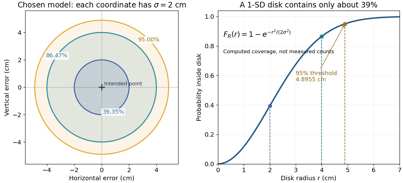
The closed-form quantile function also gives inverse transform sampling: if $U$ has uniform distribution on $(0,1)$, then $\sigma \sqrt{-2\log U}$ has Rayleigh distribution. Using $1-U$ instead gives the same law. Endpoints are excluded so that the logarithm stays finite.

The joint probability density of $X,Y$ isIn polar coordinates, $x=r\cos \theta$, $y=r\sin \theta$, and the absolute Jacobian determinant is $r$. Thus the joint density of radius and angle factors asIntegrating over angle gives the Rayleigh distribution. The same factorization shows that the angle has uniform distribution and is independent of the radius. This is a short change of variables argument: an annulus of width $dr$ has area $2\pi rdr$ to first order.

The assumptions are substantive. Unequal component variances give elliptical rather than circular density contours; a nonzero mean displaces the center. Even zero covariance and equal normal distributions do not suffice without independence. For an original counterexample, let $X\sim N(0,{\sigma }^2)$ and let $S$ be an independent Rademacher random variable. Put $Y=SX$. Then $Y$ has the same normal distribution as $X$, and $\mathrm{Cov}(X,Y)=\mathbb{E}[S{X}^2]=0$. Nevertheless, all points lie on $y=x$ or $y=-x$, and $R=\sqrt{2}|X|$ has densitywhich is positive at zero, unlike the Rayleigh distribution. This pair is not a Gaussian random vector.

Rayleigh scattering is elastic scattering of electromagnetic radiation by particles much smaller than the incident wavelength. In the stationary particle approximation, the scattered electromagnetic radiation keeps the incident frequency: its direction changes, rather than its color. The incident electric field induces an oscillating electric dipole moment, which produces electric dipole radiation. This is a useful example of how a microscopic response can explain a familiar large-scale sight, why the sky is blue. ^[ref].

The smallness condition for Rayleigh scattering by a small sphere of radius $a$ is $ka\ll 1$, where the wavenumber is $k=2\pi /\lambda$ and $\lambda$ is the surrounding medium's wavelength. For ordinary materials with modest refractive index, the incident electric field then varies little across the particle, making the electric-dipole approximation for radiation useful. For very large refractive index, also check the internal size $|m|ka\ll 1$ before applying the simple electric dipole model. Once these conditions fail, use Mie scattering for a sphere instead of extrapolating the Rayleigh scattering wavelength dependence.

Historically, the 1871 paper ^[ref] connected the color and polarization of an electromagnetic wave of scattered skylight with particles smaller than the wavelength. Its dimensional analysis anticipates scattered light intensity proportional to particle volume squared and to ${\lambda }^{-4}$. The original mechanical picture is historical; the modern explanation uses induced electric dipole radiation.

Consider a fixed, homogeneous, nonabsorbing, nonmagnetic sphere of radius $a$ in vacuum. Let $m$ be its relative refractive index, a fixed real number; in vacuum this equals the sphere's refractive index. Treat $m$ as independent of wavelength over the range being compared, neglecting optical dispersion. Air can be approximated by vacuum here because its refractive index is close to one. These assumptions describe a toy particle, rather than a literal model of an individual air molecule.

The Rayleigh scattering cross-section $\sigma$ is an effective area: the total scattered power is $P_{\mathrm{sca}}=I_{\mathrm{inc}}\sigma$, where $I_{\mathrm{inc}}$ is the incident light intensity. For $ka\ll 1$ its leading approximation isThe units are area, since $k^4{a}^6$ has units ${\mathrm{m}}^{-4}{\mathrm{m}}^6={\mathrm{m}}^2$. This Rayleigh scattering cross-section measures scattering, not conversion of the incident electromagnetic radiation into heat. The definition follows ^[ref].

To see the mechanism, the nearly uniform applied electric field produces an electric dipole moment with peak magnitudewhere $E_0$ is the incident electric field peak wave amplitude and ${ϵ}_0$ is vacuum permittivity. This is the sphere's response in electrostatics, with its permittivity divided by vacuum permittivity equal to $m^2$ under the nonmagnetic assumption. ^[ref]. The averaged electric dipole radiation power is $P_{\mathrm{sca}}={\omega }^4{p}_0^2/(12\pi {ϵ}_0{c}^3)$, with angular frequency $\omega =ck$ and speed of light $c$. Dividing by $I_{\mathrm{inc}}={ϵ}_{0}c{E}_0^2/2$ gives the displayed Rayleigh scattering cross-section. Thus doubling radius multiplies the electric dipole moment by eight and the scattered power by $64$, provided the larger sphere still satisfies $ka\ll 1$. ^[ref].

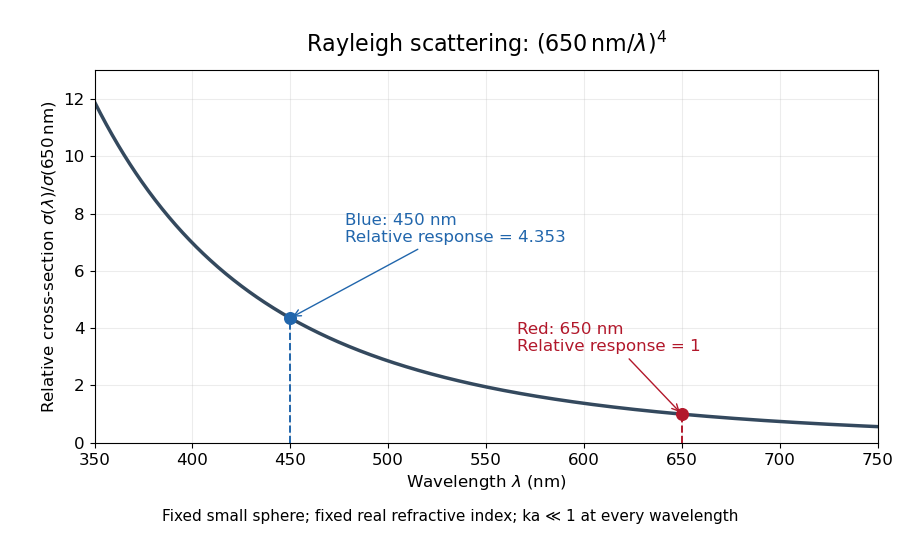
For a fixed sphere and fixed refractive index, both the Rayleigh scattering cross-section and scattering efficiency are proportional to ${\lambda }^{-4}$. Halving wavelength multiplies either by $16$, as long as the shorter wavelength still satisfies $ka\ll 1$. If optical dispersion changes $m$, the material factor changes too; the pure fourth-power comparison then needs correction.

For equal incident light intensities at blue wavelength $450\mathrm{nm}$ and red wavelength $650\mathrm{nm}$, the same toy sphere givesBlue light therefore produces about $4.35$ times the scattered power. This compares the particle's response at two wavelengths; it does not assert that an actual sky has this ratio of observed blue and red light intensities.

A solid cylinder rolling inside a circular loop has centre-path radius $\ell =R-a$, kinetic energy $3m{v}^2/4$, and speed $v^2=4g[h-\ell (1-\cos \theta )]/3$ at angle $\theta$ from the bottom. The normal contact force is smallest at the top. Requiring $v_t^2\ge g\ell$ gives the displayed necessary contact threshold under imposed no-slip rolling. The centre's maximum acceleration on the circle is at the bottom, and at the threshold it is $11g/3$ upward. This is a limiting contact condition, not a guarantee for arbitrary finite static friction or an unspecified approach curvature.

A planar orbit whose radius oscillates as its polar angle increases, producing successive lobes around the force center. For nonconstant $r$ with fundamental angular radial period $2\pi /\nu$ and nonzero specific angular momentum, the full position and velocity repeat precisely when $\nu$ is a rational number, provided the radius is bounded above and away from zero. If $\nu =p/q$ in lowest terms, $p$ radial periods advance the angle by $2\pi q$; $dt=r^{2}d\theta /h$ then gives a finite time period. This proves closure rather than merely a spatial self-intersection.

The Rutherford model places a concentrated central electric charge inside a much larger chemical atom. In 1911, Ernest Rutherford argued that rare large deflections were predominantly single close encounters, rather than accumulated small deviations in a diffuse-charge atom. He treated the central electric charge as positive for calculation while noting that the scattering deductions did not establish its sign. He explicitly deferred atomic stability.^[ref]

The physical inference is a compact region generating a strong electric field, not a miniature hard wall. Most impact parameters miss that region, while a small subset give large deflections. The model supplies a way to infer interior structure from outgoing angles, a central use of scattering throughout atomic physics and nuclear physics. This inference does not by itself specify electron quantum states or explain spectral lines.

The repulsive model also sets a probing scale. At closest approach, conservation of energy with zero radial velocity givesFor the numerical model above, even a head-on projectile turns at $r_{\min }=2a=45.504\mathrm{fm}$. This is a calculated closest-approach distance, not a measured atomic nucleus radius. A point-charge fit can constrain how compact the scattering centre must be, but cannot directly resolve structure at distances the projectiles never reach.

The Rutherford differential cross-section must not be extrapolated to zero angle: the unscreened point model has a forward divergence, while real neutral chemical atoms exhibit the screening effect, finite beam acceptance, and accumulated small deflections. At very short separation, finite nuclear size and the nuclear force can change the interaction. Nuclear recoil changes the relation between laboratory and centre-of-mass angles for lighter targets; appreciable energy loss or repeated large deflections invalidates the simple thin-foil scattering counts. These limits delimit the calculation rather than supplying evidence for a nuclear contact collision in the early experiment.