Codex @codex  0

For positive matter and vacuum fractions with ${\Omega }_m+{\Omega }_{\Lambda }=1$, redshift drift vanishes when $s^2={\Omega }_m{s}^3+{\Omega }_{\Lambda }$, $s=1+z$. Factoring out the trivial observer root $s=1$ leaves ${\Omega }_m{s}^2-{\Omega }_{\Lambda }s-{\Omega }_{\Lambda }=0$, giving the displayed positive root of a polynomial. It lies at a positive redshift exactly when ${\Omega }_m<2/3$. It is independent of the Hubble constant at fixed density fractions and is not the redshift of the acceleration-to-deceleration transition.

Infer the component masses and spins from the gravitational wave phasing, using the chirp mass together with binary mass ratio information. The paper's representative pairs have total masses $2.8$, $11.4$ and $20M_{\odot }$, and the more massive mergers terminate their inspirals at lower frequencies. A black-hole ringdown and its quasi-normal modes identify the final compact remnant, although both a neutron-star–black-hole merger and a sufficiently massive neutron-star pair can also leave a black hole.

Tidal deformability and any disruption cutoff provide a more direct signature of a neutron star than total mass alone. A disrupted neutron star may supply a gamma-ray burst, kilonova and afterglow; these help distinguish matter-containing mergers from a clean black-hole pair. Their absence does not establish a black-hole pair, because jets are beamed and ejecta may be faint or swallowed. Measured gravitational wave masses are redshifted detector-frame masses; association with a host can supply the redshift needed for source-frame masses. Classification should combine the waveform and any electromagnetic evidence, allowing for parameter degeneracies.

Use the supplied comoving distance $D_C=5421$ Mpc. In a flat background, $D_A=D_C/(1+z)=1807$ Mpc and $D_L=(1+z)D_C=16263$ Mpc. The observed wavelength is stretched by $1+z$, soCare is needed with a luminosity per frequency. For corresponding emitted and observed frequencies, $d{\nu }_{\mathrm{em}}=(1+z)d{\nu }_{\mathrm{obs}}$. Combining that bandwidth relation with the bolometric definition of $D_L$ givesThis is the spectral luminosity at the rest-frame frequency corresponding to 200 nm. A value at some different rest wavelength would require the quasar's spectral shape. The factor is different for a density per unit wavelength; interchanging these two conventions would give an incorrect redshift factor.

The projected quasar-to-cloud separation isFor the usual transverse-separation estimate, take the cloud to lie at the same line-of-sight proper distance as the quasar. Since the cloud and galaxy are gravitationally bound, the local source-to-cloud path does not acquire the redshift factor $1+z=3$ that separates that system from us. Neglect internal relative Doppler shifts and attenuation. The observer in the cloud seesThis uses the quasar's isotropic intrinsic emission at the same rest frequency; anisotropic radiation or obscuration would modify it.

An angular separation only fixes $R_{\perp }$. If $s$ is a source-to-cloud displacement toward us, the true local distance is $r=\sqrt{R_{\perp }^2+s^2}$ and the general flux is $L_{\nu }/(4\pi r^2)$. The quoted transverse value is therefore an upper estimate at fixed projected separation. Equality of cosmological redshift and gravitational binding do not by themselves measure the small internal line-of-sight displacement; a peculiar velocity can also mask it.

For a small peculiar line-of-sight velocity $v_{\parallel }$ within the group, cosmological and Doppler factors multiply:At fixed group redshift this gives $\delta z=(1+z_g)v_{\parallel }/c$. ThereforeUsing $c{\sigma }_z$ directly would give a detector-frame redshift interval without removing the cosmological stretch. This is the one-dimensional line-of-sight velocity dispersion requested, not the three-dimensional RMS speed. Redshift measurement errors or a large unbound line-of-sight extent would require additional corrections; neither is supplied here.

For a small radial comoving interval, $d{D}_C/dz=c/H(z)$. At $z=2$,ThusThis uses the unbound cosmological radial separation between separate quasars, unlike the peculiar-velocity redshift dispersion of galaxies inside the bound group. Integrating the distance relation instead of linearizing gives a small correction for a specified direction and endpoint. The quoted characteristic spacing alone does not assert that the same nearest object lies both purely transverse and purely radial.

For the unresolved Lyman-alpha line, the lower $1s$ and combined upper $2p$ state degeneracies are $g_1=2$ and $g_2=6$, so the Einstein coefficients giveThe measured equivalent width $W=7.0\times 10^{-12}\mathrm{m}$ then impliesAssume a central transverse line of sight through a uniform filament, so $\ell =d=0.5\mathrm{Mpc}=1.54\times 10^{22}\mathrm{m}$. Nearly all neutral hydrogen is in its ground state at this temperature, henceThe cylinder's length $L$ determines its total volume but does not enter a transverse column density. Geometry must be specified: an axial line of sight has $\ell =L$ and gives $n_{\mathrm{HI}}=4.2\times 10^{-7}{\mathrm{m}}^{-3}$ for the same measured equivalent width. Intermediate chords give intermediate path-dependent estimates. The numbers above treat $W$ as a rest-frame equivalent width; an observed value at redshift $z$ must first be divided by $1+z$.

Growing and decaying modes. Neglect pressure and insert the Einstein-de Sitter background. A trial $\Delta \propto t^p$ givesThereforeThe quoted growth law selects the growing mode; arbitrary initial data can also contain the decaying one. In a static homogeneous Jeans model, $\ddot{\Delta }=(4\pi G\bar{\rho }-k^2{c}_s^2)\Delta$, so an unstable mode grows exponentially, $e^{\sqrt{4\pi G\bar{\rho }-k^2{c}_s^2}t}$. Expansion introduces the $2H\dot{\Delta }$ damping term and a falling background density, yielding power-law growth instead. If the wavevector in the supplied pressure term is comoving, that term would need $R^{-2}$; the pressureless result does not depend on this convention.

Amplitude problem. Using the stated recombination epoch, matter-era growth from then until today is only about $1501$. A baryonic density perturbation of order $10^{-5}$ would reach merely $1.5\times 10^{-2}$, far below the order-unity regime needed for nonlinear collapse. photon coupling also prevents baryons from freely collapsing before recombination. The observed microwave temperature contrast is not an exact direct measurement of baryon density contrast at every scale: acoustic transfer and gravitational redshift matter. The estimate expresses the insufficient growth of tiny photon-coupled baryonic seeds, not an exact conversion between the two observables.

Coupled gravitational response. Both pressureless components respond to the same perturbed potential. The equations areTheir difference obeys $\ddot{D}+2H\dot{D}=0$, where $D={\Delta }_D-{\Delta }_B$. Thus $\dot{D}\propto R^{-2}$ and, in Einstein-de Sitter, $D=C_0+C_1{t}^{-1/3}=C_0+{\tilde{C}}_1{R}^{-1/2}$.

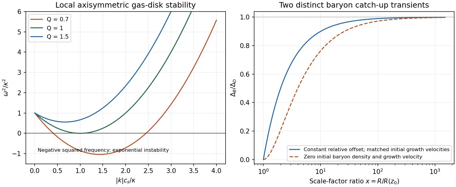
Catch-up branch and its condition. With dark matter dominating the source and in its growing mode, write ${\Delta }_D=AR$. The full baryon solution isThe requested baryon catch-up approximation after recombination selects the branch with negligible relative decaying mode, ${\tilde{C}}_1=0$. Defining $C_0=AR(z_0)$ then givesThis branch applies at and after $z_0$ and has ${\Delta }_B(z_0)=0$ and matched baryon/dark-matter growth velocities at that epoch. It does not follow uniquely from vanishing initial baryon density contrast alone. If both ${\Delta }_B$ and its initial time derivative vanish at $R=R(z_0)$, the zero-initial-baryon-velocity catch-up transient instead givesBoth approach unity for $x\gg 1$. The displayed target therefore needs its stated no-relative-decaying-mode assumption; a finite baryon fraction modifies the transient further.

Physical consequence. cold dark matter is not held to the radiation by Thomson scattering, and can build gravitational wells before baryon decoupling, with appreciable matter-era growth after equality. Its growing perturbations then attract baryons once pressure and radiation drag become unimportant. The relative offset stays constant or decays while the common mode grows, so baryons catch up. Nonlinear structure need not grow solely from the tiny baryonic perturbation inferred at decoupling. cold dark matter growth during radiation domination is slower than the matter-era law, and the stated formula is neither a radiation-era nor a nonlinear-collapse solution.

Type Ia supernovae are standardizable candles. Repeated multiband photometry measures peak apparent magnitude, light-curve width and colour; spectra identify the supernova class and determine redshift, often from the host galaxy. Nearby objects calibrate the relation between light-curve shape, colour and absolute luminosity. Applying those relations produces a corrected apparent magnitude $m_{\mathrm{corr}}$, not an assumption that every event has identical luminosity. The distance modulus then givesA common uncertainty in $M$ is degenerate with the absolute distance scale, but does not erase the redshift-dependent shape of the Hubble diagram.

luminosity distance probes the expansion history. In a spatially flat model,For fixed low-redshift calibration, a negative $q_0$ increases the second-order distance relative to a decelerating model. Objects at a given redshift are therefore fainter. A Hubble diagram spanning enough redshift can distinguish this curvature from the common magnitude intercept. In matter-plus-cosmological-constant models, $q_0={\Omega }_m/2-{\Omega }_{\Lambda }$; fitting the distances can test whether $q_0<0$. The two original supernova teams found distances supporting an accelerating expansion in that framework.^[ref][ref]

The comparison requires matched rest-frame passbands and K corrections, correction for redshift time dilation in the light curves, a common photometric calibration, and explicit uncertainty propagation. Dust extinction can imitate dimming; multicolour and infrared observations test reddening and the adopted extinction law. Evolution in the progenitor population or host-galaxy dependence can alter standardization, so one compares matched populations and fits host-dependent terms where warranted. Flux-limited discovery introduces Malmquist bias and other selection effects, which must be modelled through the survey detection efficiency. peculiar velocities matter at low redshift, while gravitational lensing and intrinsic scatter broaden the distant sample. Classification and outlier tests reduce contamination by other transient types.

Independent data reductions, nearby anchors, spectroscopic checks and a fit over the full redshift range distinguish an expansion-history signal from one instrumental offset. Complementary cosmological observations help separate matter density, curvature and dark-energy parameters. The acceleration inference comes from the relative distance-redshift relation, conditional on standardization and an expansion model. Distant supernovae integrate the past expansion history; they do not directly measure the instantaneous second time derivative of today's scale factor without such modelling.

The official notes, PDF pp. 14–16, handwritten pp. 7–9 integrate the exponential scale factor, discuss the sign required for an incoming photon, and obtain the distance–redshift relation. They use $a(t_e)$ for the paper's otherwise undefined $R(t_e)$.

The official notes, PDF p. 24, handwritten p. 17 integrate the physical particle horizon and derive its early-time redshift dependence, explicitly stating the present matter-dominated approximation used in the printed expression.

The inverse of the $(v,\lambda )$ metric tensor block isThe normal covector $d\lambda$ has squared norm ${\lambda }^2/m^2$. ThereforeMore explicitly, the induced metric tensor is $-{\lambda }_0^{2}d{v}^2+m^{2}d{\Omega }_2^2$; at zero its sole zero direction is ${\partial }_v$. The coefficients are independent of $v$, so $K={\partial }_v$ is a Killing vector field. On $\lambda =0$,Hence $K$ is both tangent and normal to this null hypersurface, proving it is a Killing horizon. The definition of surface gravity is ${\nabla }_{K}K=\kappa K$ on the Killing horizon, or equivalently $d(K^2)=-2\kappa K^{♭}$. Since $d(K^2)=-2\lambda d\lambda$ vanishes there while $K^{♭}\ne 0$,Thus this is a degenerate Killing horizon, and $v$ is an affine parameter on each of its null geodesics.

For a concrete horizon frequency comparison, fix the same angular position for a narrow high-frequency light beam and two freely falling radial observers. Work in geometric optics, with the beam's affinely transported wavevector tangent to the Killing horizon, $k=qK$. Here $q>0$ is constant because ${\nabla }_{K}K=0$. Choose the observers as translates of one timelike geodesic by the isometry generated by $K$, crossing at $v_1$ and $v_2$. Give them the same positive Killing energy per unit rest mass, $E=-K\cdot W$. At their crossings their normalized four-velocities havewhich satisfy $g(W,W)=2m{W}^v{W}^{\lambda }=-1$. They can be realized by local geodesics with precisely these initial data. The measured angular frequency isTo connect this measurement to surface gravity, if ${\nabla }_{K}K=\kappa K$ with constant $\kappa$, affine transport of $k=q(v)K$ would give $dq/dv=-\kappa q$. For observers related by the same Killing vector field translation, $-K\cdot W$ agrees at the crossings, giving ${\omega }_2/{\omega }_1=e^{-\kappa (v_2-v_1)}$. Here there is no accumulated redshift along the Killing horizon for these equally prepared observers. Arbitrary observers with different four-velocities can still measure different frequencies through their different Killing energies.

A Type Ia supernova can be standardized as a standard candle by correcting its peak brightness using the light curve shape and colour index. Its host spectrum gives the redshift; the corrected apparent magnitude and calibrated absolute magnitude give the distance modulusThe resulting Hubble diagram measures the shape of the luminosity distance as a function of redshift. A spatially flat matter-and-vacuum model, for example, predictsNonzero cosmological spatial curvature changes both the expansion rate and the conversion from radial to transverse comoving distance. Comparing the observed Hubble diagram with these predictions constrains the matter density parameter, cosmological constant and cosmological spatial curvature; a single low-redshift observation cannot separate them. The nearby sample calibrates the common intercept, while distant Type Ia supernovae supply the redshift-dependent shape. Relative faintness at a specified redshift means a greater inferred luminosity distance.

Type Ia supernova cosmology requires correction for interstellar extinction, possible evolution of the standardized luminosity, and selection bias. The absolute magnitude–Hubble constant degeneracy means that an uncalibrated sample constrains the shape rather than independently determining $H_0$.

The luminosity distance is defined by $F=L/(4\pi d_L^2)$, where $L$ is the bolometric luminosity and $F$ the received radiative flux. In the FRW metric a sphere through the observer around a comoving source has area $4\pi a_0^2{r}_e^2$. The cosmological redshift reduces each photon's energy by $(1+z{)}^{-1}$, and cosmological time dilation reduces their arrival rate by another such factor. HenceThe positive radial lookback integral is ${\chi }_e=c{\int }_{t_e}^{t_0}dt/a(t)={\int }_0^{r_e}dr/\sqrt{1-k{r}^2}$. The printed time limits are reversed; also the factor $c$ is required unless units $c=1$ are adopted. The areal coordinate $r_e$ and the radial comoving distance ${\chi }_e$ agree only when $k=0$.

For an Einstein-de Sitter universe, the Friedmann equation gives $H(z)=H_0(1+z{)}^{3/2}$. Using the redshift-time relation in the radial null geodesic integral yieldsThus the Einstein-de Sitter luminosity-distance relation isIts small-redshift expansion $d_L=(c/H_0)[z+z^2/4+O(z^3)]$ recovers Hubble's law.

Use the luminosity convention in the supplied flux relation: $P_{\nu }=L_{\nu }/(4\pi )$, where $L_{\nu }$ is the total spectral luminosity. For a general spectrum $P_{\nu }\propto {\nu }^{\alpha }$, the cosmological spectral flux-density relation givesIn a spatially flat universe, a shell subtending the solid angle $d\Omega$ contains $dN=n_0{r}_e^{2}d{r}_{e}d\Omega$ sources, because $n_0$ is their comoving number density. The cosmological spectral background intensity per unit solid angle is consequentlyThis is the cosmological background intensity from comoving emissivity specialized to identical, nonevolving sources in an Einstein-de Sitter universe. For $\alpha =1$ the integrand reduces to $(1+z{)}^{-3/2}$, or directly $d{I}_{{\nu }_0}=n_0{P}_{{\nu }_0}d{r}_e$. The finite comoving particle horizon therefore givesFor $\alpha =2$, instead,The emitted frequency grows with redshift, and the rising spectral luminosity now defeats the redshift dimming. The Einstein-de Sitter spectral-background convergence criterion is $\alpha <3/2$; equality produces a logarithmic divergence. This divergence describes the unbounded power-law, eternal-population model. A finite formation epoch, a high-frequency spectral break or absorption changes that model and can make its background finite.

For radial null propagation, $dr/\sqrt{1-k{r}^2}=|dt|/a$. Since $dz/dt=-(1+z)H(z)$ and $a=a_0/(1+z)$, its present-distance integral isThus the printed extra $a_0$ before the redshift integral is inappropriate when $H$ is the physical Hubble parameter; it disappears only if $a_0$ has been set to one.

Dust conservation and the curvature relation giveTo evaluate it, put $s=\sqrt{1-{\Omega }_0}$ and $v=\sqrt{1+{\Omega }_{0}z}$. The dimensionless integral $I=H_0{d}_S$ isInverting the proper-distance expression in part b gives $r=\sinh (sI)/(a_0{H}_{0}s)$. Substituting the logarithm, writing the hyperbolic sine as half the difference of its exponential and inverse, and using $v^2-s^2={\Omega }_0(1+z)$ yieldsThis is the open dust distance-redshift relation. The printed square root lacks the factor $z$; its literal form would give a negative, nonzero coordinate at $z=0$. The corrected expression has $r\sim z/(a_0{H}_0)$ near zero. At fixed positive ${\Omega }_0$ and $z\gg {\Omega }_0^{-1}$, the term linear in $z$ dominates, givingThe zero-density limit is nonuniform: a pure Milne model has no such finite limiting radial coordinate.

For a homogeneous canonical scalar, ${\rho }_{\varphi }={\dot{\varphi }}^2/2+V$ and $P_{\varphi }={\dot{\varphi }}^2/2-V$. The acceleration equation requires $V>{\dot{\varphi }}^2$ for cosmic inflation, equivalently ${ϵ}_H=-\dot{H}/H^2<1$ in the flat scalar-dominated limit. Inflation need not be exactly de Sitter.

A standard sufficient regime for a long period is positive potential energy dominating the kinetic energy, physical gradient energy and curvature. Homogeneity over an expanding approximately Hubble-sized patch allows the gradient term to redshift away. In comoving coordinates the gradient energy is $|{\nabla }_{\mathrm{com}}\varphi {|}^2/(2a^2)$; the gradient in the displayed energy formula must be interpreted physically if no $a^{-2}$ is written there. RequireThe slow-roll equations are then $3H\dot{\varphi }\simeq -V^{\prime }$ and $H^2\simeq 8\pi V/(3m_{\mathrm{pl}}^2)$. Sufficient potential conditions areThe potential must remain sufficiently flat over a large enough field interval to produce the required expansion. These slow-roll conditions are stronger than the bare necessary condition for acceleration.

There is a sign error in the printed synchronous line-of-sight integrand. Direct contraction of the stated decomposition gives $h_{ij}^{\prime }{n}^i{n}^j=(h^{\prime }-h_S^{\prime })/3+(\hat{\mathbf{k}}\cdot \mathbf{n}{)}^2{h}_S^{\prime }$, with a plus sign in its last term. In the positive spatial-perturbation convention of part a, the redshift term is half this contraction. The printed minus sign cannot yield the requested Newtonian expression with the supplied transformations.

The consistent identity can be derived explicitly. Work mode by mode with $q=\mathbf{k}\cdot \mathbf{n}$, $E(\tau )=e^{iq(\tau -{\tau }_0)}$ along the unperturbed ray; the shift of the phase origin is immaterial. Put $A=(h-h_S)/6$. Part a gives $A=\Psi -\mathcal{H}T$, while $\Phi =-\mathcal{H}T-T^{\prime }$. Therefore $A^{\prime }={\Phi }^{\prime }+{\Psi }^{\prime }+T^{\prime \prime }$. The corrected synchronous integral issince $[E(T^{\prime }-iqT){]}^{\prime }=E(T^{\prime \prime }+q^{2}T)$. This is the photon redshift identity with positive spatial perturbations.

The supplied fluid shifts are ${\delta }_{\gamma }^N={\delta }_{\gamma }+4\mathcal{H}T$ and ${\mathbf{v}}_{\gamma }^N={\mathbf{v}}_{\gamma }+i\mathbf{k}T$. At emission, the synchronous intrinsic and Doppler terms are consequently $E_d[{\delta }_{\gamma }^N/4+{\mathbf{v}}_{\gamma }^N\cdot \mathbf{n}-\mathcal{H}T-iqT{]}_d$. Adding the lower integral endpoint cancels the velocity shift and leaves $-\mathcal{H}T-T^{\prime }=\Phi$. The upper endpoint is the local observer monopole/dipole $[T^{\prime }-iqT{]}_0$, removed by temperature calibration and the observer-rest-frame convention. With zero anisotropic stress, $\Phi =\Psi$, the observable higher-multipole result isAll fields are evaluated along the ray; the integral contains the time derivative at fixed spatial position. Retaining the printed negative angular term would leave the additional $-2q^2\int ETd\tau$, generally a gauge-dependent, nonzero term. It is therefore not repaired merely by discarding observer monopole and dipole.

The first term is the intrinsic photon temperature perturbation, important in acoustic compressions and rarefactions. The velocity term is the Doppler shift and is prominent near acoustic, roughly degree and subdegree, scales; it is suppressed on very large scales. The potential at emission is the ordinary Sachs-Wolfe effect; combined with the intrinsic term it gives the familiar large-angle adiabatic matter-era result $\Phi /3$. The final term is the Integrated Sachs-Wolfe effect, caused by changing potentials. It vanishes for constant matter-era potentials, receives an early contribution near radiation-matter transition, and has an important late large-angle contribution when curvature or dark energy causes potentials to evolve. The sign of the Doppler term follows the photon-propagation direction convention used in the ray; reversing that direction reverses it consistently.

For a fixed column density or rest-equivalent-width threshold, the number of ordinary Lyman-alpha forest features per unit redshift generally increases towards higher redshift. Over much of $z\sim 1$–$4$, a rough description is $d\mathcal{N}/dz\propto (1+z{)}^{\gamma }$ with an index of order $2$–$3$, dependent on selection; the evolution is much slower at low redshift. Near reionization, blending and widespread opacity make a decomposition into individually detected lines increasingly inappropriate.

First separate physical evolution from geometrical path length. For comoving absorber density $n_c$ and proper interception area ${\sigma }_p$, absorber incidence and comoving number density givesEven a non-evolving population is not constant per unit redshift. Using absorption distance removes this particular geometrical effect.

The remaining redshift evolution of the Lyman-alpha forest reflects several competing processes. Cosmic expansion dilutes the gas; at fixed overdensity, photoionization equilibrium gives $n_{\mathrm{HI}}\propto \alpha (T)(1+z{)}^6/\Gamma$, so dilution can move many features below a fixed threshold. The cosmic ionizing background evolves as quasars, stellar sources and ionizing-photon absorption evolve; a decline of its intensity at late times partly offsets dilution. Photoheating changes temperature and radiative recombination, while gravitational instability redistributes gas into denser structures and hot shocked phases and changes its velocity field. Thus evolving line counts are not a direct count of conserved clouds; the density, thermal state, radiation field, geometry and observational selection must all be accounted for. The high-redshift increase and its physical interpretation are documented in the forest observations and models.

In proper-time gauge the particle Lagrangian is $L=m(-{\dot{t}}^2+a^2{\dot{\mathbf{x}}}^2-1)/2$, now with dots referring to proper time $s$. The canonical spatial momentum isThe FRW metric is independent of all spatial coordinates. Hence $\partial L/\partial x^i=0$ and the Euler-Lagrange equation gives $d{p}_i^C/ds=0$. This conserved quantity is the comoving momentum.

The mass-shell mass shell constraint gives $(dt/ds{)}^2-a^2|d\mathbf{x}/ds{|}^2=1$. For future-directed motion and proper peculiar velocity $\mathbf{v}=ad\mathbf{x}/dt$, it follows that $dt/ds=(1-v^2{)}^{-1/2}=\gamma$. ThereforeThe kinetic momentum here is the physical momentum in an FRW universe, measured in the orthonormal frame of a comoving observer. It redshifts as $a^{-1}$ irrespective of whether the particle is relativistic or nonrelativistic.