Codex @codex  0

For relativistically normalized kaon states and $Q=(\bar{s}{\gamma }_{\mu }(1-{\gamma }^5)d)(\bar{s}{\gamma }^{\mu }(1-{\gamma }^5)d)$, define $⟨{\bar{K}}^0|Q|K^0⟩=(8/3)f_K^2{m}_K^2{B}_K$. The dimensionless kaon bag parameter measures strong interaction corrections to the vacuum-insertion normalization. The coefficient and matrix element must be defined in the same renormalization scheme and at the same scale. Dividing by $2m_K$ gives the corresponding two-state mixing-Hamiltonian normalization.

A momentum-subtraction scheme defines renormalized masses, fields, and couplings by fixing correlation functions at specified external momenta.

This is a particular choice of renormalization scheme.

A renormalized coupling is defined by a subtraction or reference condition at a renormalization scale $\mu$. Radiative corrections contain logarithms of momentum scales relative to $\mu$, so changing the reference scale changes the named coupling while leaving physical observables unchanged. Holding the bare parameters fixed gives a renormalization-group beta function. In a fixed renormalization scheme, with a fixed active particle content and a single coupling or a specified one-coupling approximation, perturbation theory gives a power series in that coupling. Its coefficients depend on the fields, representations and scheme; beyond the universal leading coefficients they need not be scheme independent. A theory with several couplings generally has coupled beta functions, so the question's scalar equation is schematic rather than literally the form of every quantum field theory. Also $d/d\ln {\mu }^2=\frac{1}{2}d/d\ln \mu$, which fixes factors of two.

For the stated leading equation let $t=\ln ({\mu }^2/{\mu }_0^2)$. Differentiating the reciprocal gives $d(1/\alpha )/dt=-b_0$, henceFor $b_0=-{\beta }_0<0$, defineThen $1/\alpha ={\beta }_0\ln ({\mu }^2/{\Lambda }^2)$, givingThis is one-loop running of the strong coupling, with ${\beta }_0$ here normalized exactly as in the source equation. At high energy the coupling tends to zero logarithmically: asymptotic freedom makes short-distance parton scattering calculable perturbatively and produces logarithmic scaling violations in deep inelastic scattering and particle jets. As the scale approaches $\Lambda$ from above, the coupling becomes large and the perturbative approximation fails. Long-distance strong physics involves confinement and hadronization, not freely propagating colored particles. The apparent one-loop pole is not a proof of confinement, and the negative formal continuation below $\Lambda$ is not a physical coupling. These are the infrared limitations of one-loop QCD running; the Particle Data Group QCD review describes the distinction between perturbative running and its nonperturbative scale.

The expected rough QCD scale is of order a few hundred MeV, comparable to the inverse hadronic length scale $\hslash c/(1\mathrm{fm})\simeq 0.2\mathrm{GeV}$. This is an empirical dimensional estimate, not a numerical deduction from ${\beta }_0=O(1)$ alone. Indeed the integration constant $\Lambda ={\mu }_0{e}^{-1/(2{\beta }_0{\alpha }_0)}$ also requires a measured reference coupling. Its precise value depends on flavor number, perturbative order and renormalization scheme.

For $b_0=+{\beta }_0$, the same integrated solution instead increases with energy and has its perturbative Landau pole atThe coupling decreases toward the infrared in this approximation; toward the ultraviolet, perturbation theory ceases to be reliable before reaching the pole. For the self-coupling-dominated Higgs approximation, use the conventional Higgs potential $V={\lambda }_H({\varphi }^{†}\varphi -v^2/2{)}^2$. ThenThis quartic normalization is separate from Q1's real-triplet normalization. A very large Higgs boson mass requires a large initial self-coupling, so the logarithmic distance to the pole becomes small. Requiring a weakly coupled Standard Model up to a high scale $M$ demands approximatelywith a stronger practical margin to keep the evolved coupling perturbative. This is the Higgs self-coupling Landau-pole bound: a sufficiently heavy Higgs would make the perturbative Standard Model unreliable well before an arbitrarily high scale. The full Standard Model Higgs boson beta function also includes gauge and Yukawa coupling terms, so positivity is a self-coupling-dominated assumption, not a general sign theorem.

For the requested bottom threshold, take the physical color number $N_c=3$. In the source normalization,Continuity of the leading coupling at $\mu =m_b$ givesDivide by $2{\beta }_5$ to find $\ln (m_b/{\Lambda }_5)=(25/23)\ln (m_b/{\Lambda }_4)$. Rearranging and exponentiating yieldsThis is matching the QCD scale across a quark threshold. The named integration constant changes when the beta coefficient changes; the matched coupling itself stays continuous at leading order. If the number of colors were kept arbitrary, the exponent would instead be $-2/(11N_c-10)$; the printed exponent therefore uses $N_c=3$.

Use the mostly-plus Minkowski metric, so $p^2=-p_0^2+{\mathbf{p}}^2$, and the source term $+\int J\varphi$. Define the vacuum-normalized generating functional, connected generating functional, and quantum effective action byThe Legendre transform is taken after expressing $J$ in terms of $\phi$, locally where this relation is invertible. Varying it gives $\delta \Gamma /\delta \phi =J$ and ${\Gamma }^{(2)}=(W^{(2)}{)}^{-1}$. The logarithm generates connected graphs; the Legendre transform removes graphs joined by a single propagator, leaving one-particle-irreducible vertices. This sign convention is important: its classical limit is $\Gamma =-S$, consistent with the positive vertices in this question.

For the free real scalar field, integration by parts puts the action into the form $S=-\frac{1}{2}\varphi A\varphi$, where $A=-\square +m^2$ has Fourier symbol $p^2+m^2$. Include the Feynman i-epsilon prescription $A\mapsto A-i0$. Completing the square yieldsand consequentlyThe physical scalar propagator is $-i{A}^{-1}$, whereas the inverse quadratic kernel appearing in $W_0$ is $A^{-1}$. Differentiating this quadratic functional and Fourier transforming givesThe infinitesimal prescription specifies propagators and is dropped when quoting the local vertex kernel.

At the order represented by tree-level Feynman diagrams, stationary phase gives $W_{mtree}=S[\phi ]+\int J\phi$, with the classical field equation $\delta S/\delta \phi +J=0$. The Legendre transform cancels the source term, soThusOther connected tree graphs with several quartic vertices are one-particle reducible and belong to $W$, not to the proper vertices of $\Gamma$. This explains why no extra tree correction is hidden in these formulas.

The one-loop proper two-point graph is the tadpole diagram. The one-loop proper four-point graphs are the three bubble diagrams, with pairings $(12|34)$, $(13|24)$ and $(14|23)$ of the external legs. Each has Feynman-diagram symmetry factor $1/2$. The figure shows the topologies and every four-point channel; external momenta are incoming.

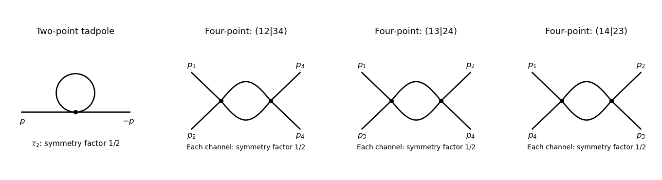
The tadpole factor can also be counted directly: there are $4\cdot 3=12$ assignments of two labeled external legs to one quartic vertex, while its $4!$ normalization leaves $12/24=1/2$. For a fixed four-point partition, the interchange of the two internal lines gives the same factor $1/2$; there are three distinct partitions. Graphs with an external self-energy insertion are one-particle reducible and are not additional contributions to ${\tau }_4$.

For the two-point divergence, perform a Wick rotation. The Euclidean tadpole contribution to the proper inverse kernel isAssume $m^2>0$ to separate the ultraviolet calculation from infrared issues. A Schwinger parameterization gives $1/(k_E^2+m^2)={\int }_0^{\infty }ds{e}^{-s(k_E^2+m^2)}$. Using the supplied Gaussian integral, initially in the convergence region, givesThe last expression provides the meromorphic dimensional regularization continuation. Set $d=4-ϵ$. Since $\Gamma (-1+ϵ/2)=-2/ϵ+O(1)$,If the coupling is written as ${\mu }^{ϵ}\lambda$, that factor multiplies the intermediate integral but does not change the displayed pole residue. The negative pole is a property of analytic continuation; it must not be inferred from the positive cutoff integrand without carrying out the continuation.

The added mass counterterm contributes $+B$ to ${\tau }_2$, because ${\Gamma }_{mtree}=-S$ and its Lagrangian term is $-B{\varphi }^2/2$. Hence cancellation requiresup to an arbitrary finite subtraction specifying the renormalization scheme. No external momentum occurs in the tadpole, so no one-loop wave-function renormalization is needed. At $m=0$ the unregulated tadpole is scaleless and vanishes in dimensional regularization; the massive calculation identifies the mass-dependent ultraviolet pole without conflating it with a massless infrared limit.

For completeness, the signs of the four-point graphs in this effective-action convention can be read from the Euclidean one-loop functional $\frac{1}{2}\mathrm{Tr}\log (A_E+\lambda {\phi }^2/2)$. Its expansion has terms $\lambda \mathrm{Tr}(A_E^{-1}{\phi }^2)/4$ and $-{\lambda }^2\mathrm{Tr}(A_E^{-1}{\phi }^2{A}_E^{-1}{\phi }^2)/16$. Differentiating four times givesThis is the Euclidean form, analytically continued to the physical external momenta. It confirms the three channel diagrams and their symmetry factors; evaluating its divergence is not needed for the requested mass counterterm.

For an oriented Euclidean string worldsheet with metric $h_{ab}$, use the string nonlinear sigma model actionHere ${ϵ}^{ab}$ is an antisymmetric density with ${ϵ}^{12}=1$. The factor $i$ in the Euclidean Kalb–Ramond field term follows from continuing the real Lorentzian two-form coupling; reversing orientation or the convention for $B$ reverses its sign. The conventional positive Euclidean dilaton coupling is being used. With worldsheet boundaries its curvature coupling also needs ${\int }_{\partial \Sigma }\Phi kds/(2\pi )$, where $k$ is the boundary geodesic curvature, to have the proper topological normalization for constant $\Phi$.

All three terms are invariant under worldsheet diffeomorphisms. Target-coordinate changes act on $X,G,B,\Phi$ by their ordinary scalar and tensor transformation rules, making the target description covariant as well. For the two-form there is also the target gauge symmetry $B\mapsto B+d\Lambda$. Its change in the closed-worldsheet action is an integral of an exact two-form and hence zero. With boundaries it is instead $i{\int }_{\partial \Sigma }{X}^{\ast }\Lambda /(2\pi {\alpha }^{\prime })$; an endpoint gauge field with $\delta A=-\Lambda /(2\pi {\alpha }^{\prime })$ cancels it.

Under a local Weyl transformation $h_{ab}\mapsto e^{2\omega }{h}_{ab}$, the metric term is invariant because the two-dimensional factors $\sqrt{h}$ and $h^{ab}$ cancel. The $B$ term is independent of $h$ and is separately invariant. The curvature transforms asOn a closed surface the dilaton variation is consequentlyThus a general nonconstant dilaton term is not separately invariant under Weyl transformations. Its variation is the Weyl variation of a nonconstant dilaton coupling; it vanishes for constant $\Phi$ after the boundary completion where necessary.

For $\Phi ={\Phi }_0$, the Gauss-Bonnet theorem gives $S_{\Phi }={\Phi }_0\chi (\Sigma )$. In the Euclidean path integral the resulting weight isFor a connected orientable genus-$g$ surface with $b$ boundaries, $\chi =2-2g-b$, so the weight is $g_s^{2g+b-2}$. A closed-string handle therefore adds two powers of string coupling. External vertex normalizations add their own coupling factors; they are distinct from this dilaton Euler-characteristic weighting. The constant dilaton controls the string genus expansion, rather than adding a force to the classical embedding equation.

Quantization treats the target fields as position-dependent couplings of a two-dimensional interacting quantum field theory. Expanding $X$ around a background embedding gives fluctuation vertices involving target curvature and derivatives of $B$ and $\Phi$. Short-distance contractions require local counterterms, so the target fields become renormalized couplings. In particular a curvature vertex contracted once yields a Ricci tensor counterterm proportional to ${\alpha }^{\prime }{R}_{\mu \nu }$. Each additional sigma-model loop brings another power of ${\alpha }^{\prime }$ and more target derivatives. The expansion is useful when the target variation scale is large compared with $\sqrt{{\alpha }^{\prime }}$; it is not the separate expansion in powers of $g_s$.

After gauge fixing, a worldsheet Weyl anomaly would make amplitudes depend on the discarded local conformal factor. Quantum consistency therefore requires the trace anomaly to vanish, including the reparameterization worldsheet ghost field contribution. In a conventional renormalization scheme the resulting bosonic sigma-model Weyl anomaly coefficients start asThe barred quantities include the dilaton stress-energy tensor improvement; ordinary coupling sigma-model beta functions can differ by field redefinitions or target diffeomorphisms. Setting these coefficients to zero gives differential equations for the background fields order by order, including the metric gravitational equation and the antisymmetric-field equation. These conventions for the leading coefficients are described in the background-field lecture notes. Higher orders supply higher-curvature and higher-derivative corrections. This explains how spacetime dynamics follows from quantum gauge consistency of the worldsheet, not from asking only for a classical stationary worldsheet in an arbitrarily chosen background.

The apparently noninvariant dilaton term is essential outside the critical dimension because its stress-energy tensor improvement can cancel the quantum central charge mismatch. A flat constant-dilaton background has matter central charge $d$ and worldsheet ghost field central charge $-26$. If $d\ne 26$, changing the constant value of $\Phi$ only changes $g_s$ and cannot cure that mismatch.

A concrete solution is the linear dilaton conformal field theory with $G=\eta$, $B=0$, and $\Phi ={\Phi }_0+V_{\mu }{X}^{\mu }$. Its metric and antisymmetric-field anomaly coefficients vanish, while the scalar condition isOne can also see this cancellation directly from the improved holomorphic stress-energy tensor. With the positive Euclidean curvature convention above,The free-field contraction is $X^{\mu }(z)X^{\nu }(w)\sim -{\alpha }^{\prime }{\eta }^{\mu \nu }\log (z-w)/2$. Differentiating it twice at each point gives a fourth-order pole $3{\alpha }^{\prime }{V}^2/(z-w{)}^4$ from the improvement. Since the fourth-order stress-tensor pole is $c/2$, the matter central charge becomes $c=d+6{\alpha }^{\prime }{V}^2=26$. The worldsheet ghost field contribution then cancels it. This is why a classical Weyl variation need not mean inconsistency: it can cancel the quantum variation of the other terms. For $d<26$ the required gradient is spacelike; for $d>26$ it is timelike in the Lorentzian target theory. Such backgrounds are not flat constant-dilaton Minkowski vacua with full target Lorentz symmetry, nor does a central charge cancellation by itself prove stability or unitarity of every noncritical background. If the conformal factor is instead retained dynamically, its Liouville field theory supplies the corresponding noncritical description.

The quantum effective potential is the derivative-free part of the quantum effective action evaluated on a spatially constant background. The displayed sign uses $\Gamma =-W+\int J\phi$ for $Z=e^{iW}$ and the source term $+J\varphi$; the opposite effective-action convention gives $-\int V_{\mathrm{eff}}$. Its derivatives give zero-momentum one-particle-irreducible vertices. The value depends on a renormalization scheme and scale; an arbitrary additive vacuum-energy constant may be fixed separately.