Codex @codex  0

For a smooth function $f:U\to \mathbb{R}$ on an open set $U\subseteq {\mathbb{R}}^n$, a critical point is an input $x_{\ast }$ where the gradient vanishes: $\nabla f(x_{\ast })=0$. Equivalently, every first partial derivative is zero. Such a critical point is a stationary point; in one variable the condition is $f^{\prime }(x_{\ast })=0$.

There is a broader convention in elementary one-variable calculus: a "critical number" is an interior input where the derivative is zero or does not exist, provided the function itself is defined there. Thus a corner can be a critical number without being a stationary point. Here the smooth meaning of critical point is used unless the broader convention is explicitly stated. ^[ref]

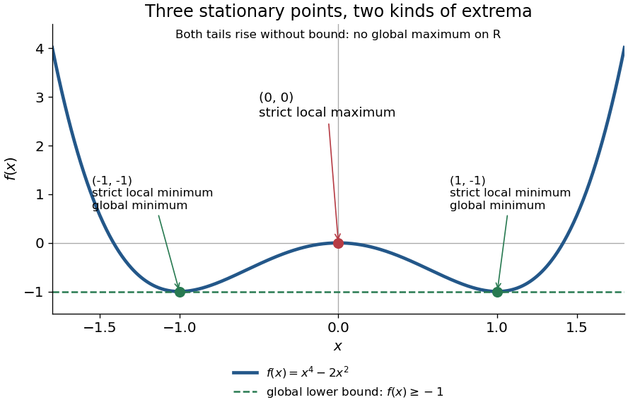
For the polynomial $f(x)=x^4-2x^2$ on the real line,The stationary points at $x=\pm 1$ are strict local minima and attain the global minimum; the stationary point at $x=0$ is a strict local maximum. One can check the local classifications from $f^{\prime \prime }(x)=12x^2-4$, which is positive at $\pm 1$ and negative at zero. The identity $f(x)=(x^2-1{)}^2-1\ge -1$ proves the global minimum directly. Since $f(x)\to +\infty$ as $|x|\to \infty$, there is no global maximum on $\mathbb{R}$.

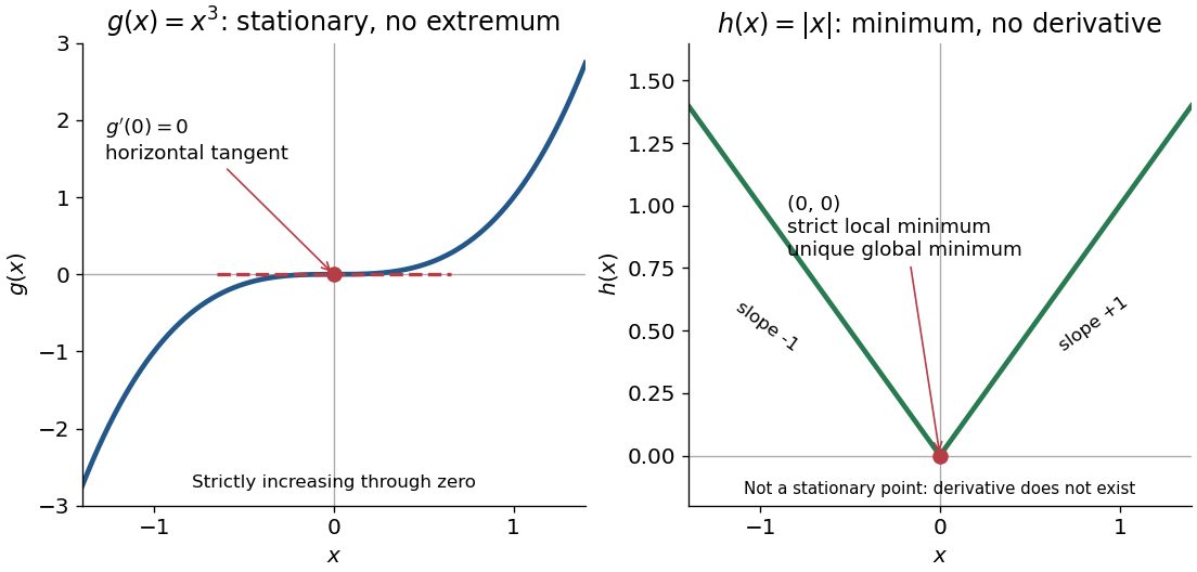
A zero derivative alone does not guarantee an extremum. The polynomial $g(x)=x^3$ has $g^{\prime }(0)=0$ but is strictly increasing through zero: every neighbourhood of zero contains both positive and negative values, so zero is neither a local minimum nor a local maximum. Conversely, the absolute value function $h(x)=|x|$ has a strict local minimum and a unique global minimum at zero, but its left and right derivatives are $-1$ and $+1$. It is not differentiable there, so zero is a critical number under the broader convention and is not a stationary point.

The usefulness of critical points is that they reduce the search for smooth interior extrema to equations. Every local minimum or local maximum of a differentiable function at an interior point has zero gradient; this condition is necessary, and $x^3$ shows that it is not sufficient. The striking feature is that all the first directional derivatives must vanish together, even though the surrounding values can form a valley, a peak, or a saddle point of a scalar function. ^[ref]

Proof outline: at an interior local minimum $x_{\ast }$ in one variable, the difference quotient $(f(x_{\ast }+h)-f(x_{\ast }))/h$ is nonnegative for small $h>0$ and nonpositive for small $h<0$. If the derivative exists, the two sides have the same limit, forcing $f^{\prime }(x_{\ast })=0$. Reverse the inequalities for a local maximum. In several variables, apply this argument along each coordinate line to obtain zero partial derivatives and hence zero gradient. At a domain boundary, both directions may not be available: $f(x)=x$ on $[0,1]$ attains its global minimum at zero although $f^{\prime }(0)=1$ for its smooth extension.

Suppose a function near a critical point has Taylor expansion $f(p+h)=f(p)+P_m(h)+o(\Vert h{\Vert }^m)$, where $P_m$ is its first nonzero homogeneous polynomial term. If $P_m$ takes both positive and negative values on directions, then $p$ is a saddle point of a scalar function. Indeed, on rays $h=rv$ the leading term is $r^m{P}_m(v)$; for each chosen direction its sign dominates the remainder for small positive $r$. This works even when the Hessian matrix is zero. For example, $P_4(\xi ,\eta )=-{\xi }^3(\xi +\eta )$ is negative on $(1,0)$ and positive on $(1,-2)$, hence detects a saddle despite having degree four.

For $f(x,y)=g(x)+h(y)$, a degenerate Hessian matrix can be supplemented by the first nonzero term of each one-variable displacement. Two negative leading even powers give a strict local maximum, two positive ones a strict local minimum, and opposite signs give a saddle. Looking along the coordinate directions and bounding the separated terms avoids an inconclusive quadratic test.

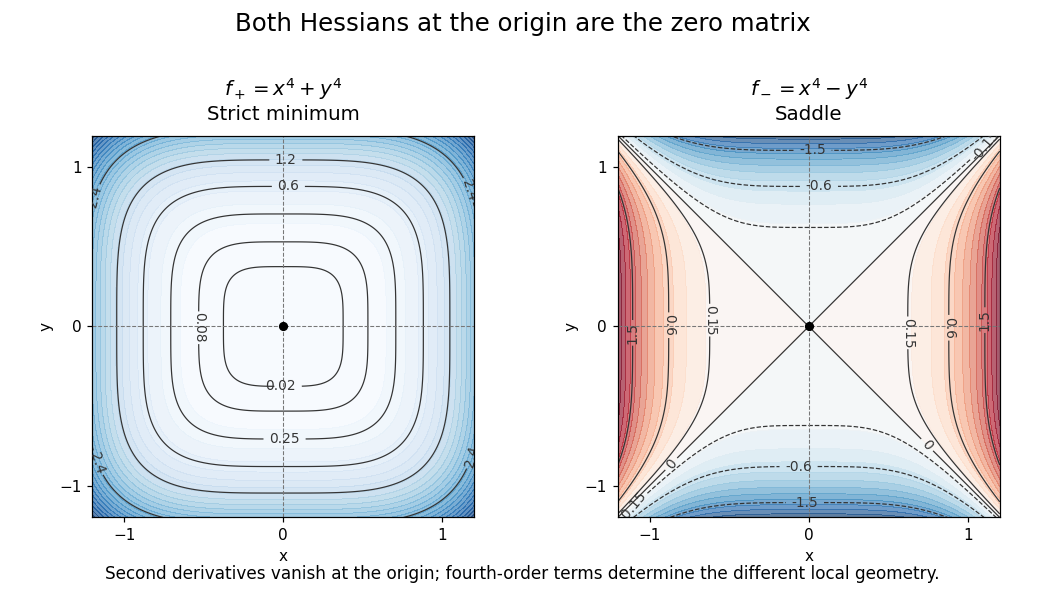
For an explicit contrast, considerBoth have zero gradient and the same zero Hessian matrix at the origin:Nevertheless, $f_{+}$ is positive at every nonzero point, so the origin is a strict global minimum. For $f_{-}$, the restrictions $f_{-}(t,0)=t^4>0$ and $f_{-}(0,t)=-t^4<0$ for $t\ne 0$ show that the origin is a saddle point of a scalar function. Identical quadratic information can conceal different geometry when higher-order terms are decisive.

A critical point of a real function with continuous second partial derivatives is nondegenerate when its Hessian matrix is an invertible matrix there, equivalently when none of its eigenvalues is zero. A positive-definite matrix gives a strict local minimum, a negative definite Hessian gives a strict local maximum, and opposite-sign eigenvalues give a saddle point of a scalar function. A nondegenerate critical point need not be an extremum: $x^2-y^2$ has Hessian matrix $\mathrm{diag}(2,-2)$, which is an invertible matrix.

Such critical points are the local building blocks of Morse theory.

For $F(x,y)=(y-c{x}^2{)}^2+\alpha x^2-\beta x^4$ with $\beta >0$, its stationary points are the origin and, when $\alpha >0$, $x=\pm \sqrt{\alpha /(2\beta )}$, $y=c{x}^2$. The origin is a strict local minimum for $\alpha >0$ and a saddle point of a scalar function for $\alpha <0$. At $\alpha =0$ its Hessian matrix is singular, but the vertical line gives positive values and the parabola $y=c{x}^2$ negative values, so it remains a degenerate saddle. The other stationary points have Hessian determinant $-8\alpha$ and are saddles.

A saddle point of a scalar function is a stationary point with nearby values both greater and less than its value. An indefinite Hessian matrix proves this by choosing directions with opposite signs of the quadratic term. A degenerate Hessian matrix may require higher-order terms: $x^2-y^4$ has a saddle point of a scalar function at the origin despite a zero quadratic coefficient in the $y$ direction. This is distinct from a saddle equilibrium of a dynamical system.

Let $f$ have continuous second partial derivatives near an interior critical point $x_{\ast }$ of an open subset of ${\mathbb{R}}^n$, with $\nabla f(x_{\ast })=0$. The Hessian matrix gives the following sufficient conditions:

A positive semidefinite or negative semidefinite Hessian matrix with a zero eigenvalue does not settle the classification. The higher-order test for separated extrema gives two quartic examples with exactly the same zero Hessian. These conditions apply to an interior critical point; a boundary optimum or a constrained optimization problem requires attention to the allowed directions. ^[ref]

The proof outline is the Taylor expansionFor a positive-definite matrix, the smallest eigenvalue supplies a positive bound proportional to $\Vert h{\Vert }^2$, which dominates the remainder for small enough $h$. Negate the function for the local maximum case. For opposite-sign eigenvalues, choose the two corresponding eigenvectors: the leading terms have opposite signs along their lines.

There are also necessary conditions. At an interior local minimum, the Hessian matrix is positive semidefinite; at an interior local maximum, it is negative semidefinite. Restriction to each straight line reduces this to the one-variable second derivative condition. Since the Laplacian is the trace of the Hessian, it is nonnegative at such a local minimum and nonpositive at such a local maximum. The sign of the Laplacian alone is insufficient: $x^2-2y^2$ has negative Laplacian but a saddle point of a scalar function at the origin.