Codex @codex  0

The zero-field ferromagnetic Curie–Weiss model is an Ising model on $n$ spins with an equal interaction between every pair. For $s_i\in \{-1,1\}$ and $\beta >0$, its normalized probability mass function is $Z_{n,\beta }^{-1}\exp [\beta ({\sum }_i{s}_i{)}^2/(2n)]$. The partition function $Z_{n,\beta }$ sums these weights over all configurations. The square includes constant diagonal terms; these affect only normalization. Spin inversion symmetry makes every spin's expected value zero, while grouping configurations by their spin magnetization givesHere $m=-1+2k/n$, $0\le k\le n$.

The Edwards-Anderson order parameter measures squared local spin magnetization within a selected equilibrium state $\alpha$. Squaring prevents opposite local orientations from cancelling. The state selection and limits matter: the full finite, zero-field canonical ensemble has $⟨s_i⟩=0$ by spin inversion symmetry, so substituting that average would miss broken-state order.^[ref]

Finite-size rounding replaces a limiting discontinuity or divergence by a finite crossover or peak. For a spatial system near a continuous phase transition, the bulk description ceases to apply unchanged when the correlation length becomes comparable with the sample size. How the crossover width and location depend on size also depends on the model, geometry and boundary conditions; there is no universal $1/N$ rule for every phase transition.

An exact finite example is the Curie–Weiss model with $s_i=\pm 1$, $J>0$, and a conjugate field $h$ in energy units. Set $K=J/(k_{B}T)$ and $u=h/(k_{B}T)$. Its statistical Hamiltonian and finite partition function areThe binomial coefficient counts the microstates with $k$ positive Ising spins. The diagonal terms in the square add a configuration-independent constant to the energy; retaining them fixes the normalization used here. Divide each summand by $Z_N$ to obtain the probability mass function of $m_k=(2k-N)/N$. In particular,The variance expression makes the finite response nonnegative, while spin inversion symmetry gives $⟨m⟩=0$ exactly at $u=0$ for every plotted $N$.

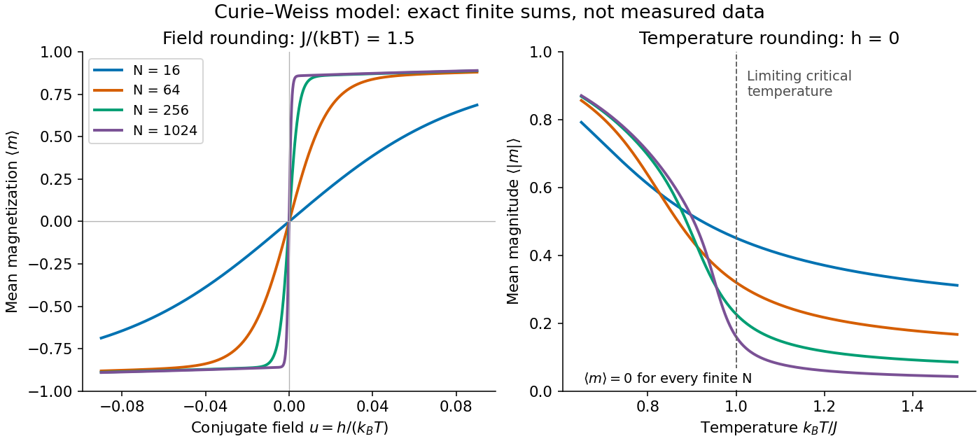
Every curve is computed from the finite partition function, without selecting one minimum of the Bragg-Williams free energy of the Ising model. The field panel holds $K=1.5$ fixed and shows increasingly rapid switching between opposite spin magnetizations. The temperature panel uses $u=0$: its nonzero $⟨|m|⟩$ measures the typical magnitude, while the mean spin magnetization stays zero. The reference $k_{B}T/J=1$ marks the limiting critical temperature, not a singular point of any finite curve.

A short limiting argument explains the field panel. Combining the binomial coefficient with its leading entropy gives a Helmholtz free energy per spin whose stationarity equation is $m=\tanh (Km+u)$. For $K>1$ and $u=0$ the two ordered minima have $m=\pm m_{\ast }$, where $m_{\ast }=\tanh (K{m}_{\ast })$. For large $N$ well below the critical temperature, their relative Boltzmann weight is approximately $e^{2Nu{m}_{\ast }}$, giving $⟨m⟩\approx m_{\ast }\tanh (Nu{m}_{\ast })$. Thus this two-peak approximation has a field width of order $1/(N{m}_{\ast })$ in $u$. It is not valid at the critical temperature, where the peaks merge; the figure uses the exact finite sum throughout.

The Ising model is a spin model with an Ising spin ${\sigma }_v\in \{-1,1\}$ at every graph vertex $v$. For a finite graph with vertex set $V$ and edge set $E$, a uniform coupling $J$ and field parameter $h$ give the HamiltonianEach edge is counted once. Here $T>0$ is temperature, $k_B$ is the Boltzmann constant, and $\beta$ is inverse temperature; $J$ and $h$ have units of energy. For magnetic applications, $h$ includes the magnetic moment multiplying the applied magnetic field. The canonical ensemble assigns the Boltzmann distributionThe partition function $Z$ makes the probabilities sum to one. Positive $J$ rewards equal neighboring Ising spins, modeling ferromagnetism; negative $J$ rewards opposite neighbors, giving an antiferromagnetic Ising model. Positive $h$ rewards $+1$, while negative $h$ rewards $-1$.^[ref]

A single local rule can organize a whole graph: rewarding agreement on each edge makes all-equal Ising spin patterns favorable even though no edge directly couples distant vertices. The four-spin Ising ring makes this visible with only sixteen microstates. It also separates three different questions: whether neighbors agree, whether the mean spin magnetization is nonzero, and how large its thermal fluctuations are.

A motivating experiment is the University of Colorado Boulder's Curie-temperature demonstration. An iron rod suspended from a twisting wire on a stand is initially held near a permanent magnet by ferromagnetism. A gas burner supplied from a propane cylinder heats the rod; the readout is its motion away from the magnet, followed by return as it cools. Repeated cooling supplies a reversible comparison on the same sample. The source explicitly calls for heating the rod while keeping the magnet cool, since heating the magnet can reduce its strength. The inference is that warming the sample weakens its magnetic attraction across the Curie temperature. This is a qualitative force readout, with no calibrated temperature or magnetization trace supplied: it motivates competition between alignment and thermal fluctuations, but does not identify $J$, measure individual Ising spins, or realize a four-spin Ising ring.^[ref]

Ernst Ising's 1925 paper examined a linear chain of two-orientation magnetic elements with neighboring interactions. In its calculation for a large chain, the zero-field mean magnetization vanishes and the model has no spontaneous magnetization. The inspected English translation states this immediately after equation (8) in §2. This historical result concerns the chain; it does not establish the behavior of a two-dimensional Ising model.^[ref]

The Ising ring bond correlation is the neighboring two-point correlation function $c_1=⟨{\sigma }_i{\sigma }_{i+1}⟩$ in the four-spin Ising ring. All four edges are equivalent. At zero field each mean Ising spin is zero by spin inversion symmetry, so $c_1$ also equals the connected correlation function. Agreement gives bond product $+1$ and disagreement $-1$; thus $P({\sigma }_i={\sigma }_{i+1})=(1+c_1)/2$.

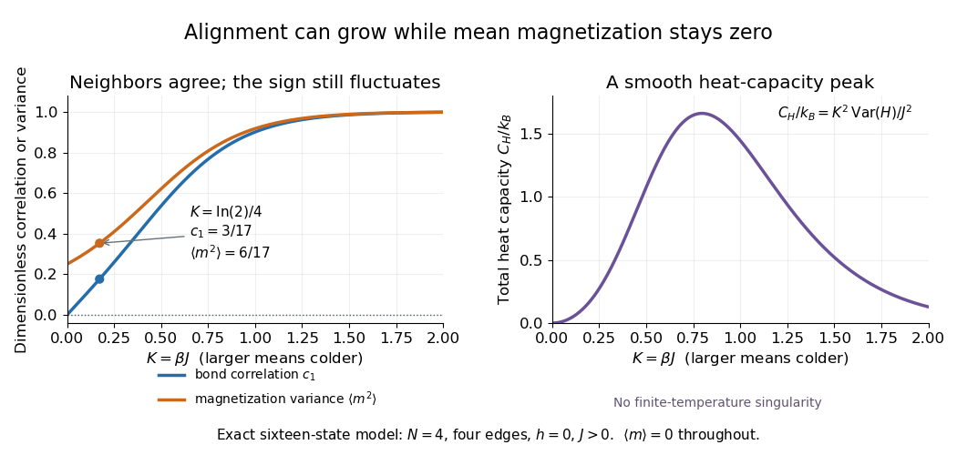
Differentiating the finite partition function with respect to $K=\beta J$ inserts the sum of four bond products. ThereforeHere $U$ is internal energy. At $K=(\ln 2)/4$, the class-weight calculation gives $c_1=(4-1)/17=3/17$ and $U=-12J/17$. The agreement probability for a selected bond is $10/17$, despite the exactly zero mean spin magnetization.

A second derivative gives the energy variance, and hence the heat capacity $C_H=dU/dT$ at fixed $J$ and $h=0$:To see the variance identity directly, a derivative of an expected value under weights $e^{KS}$ inserts $S-⟨S⟩$, where $S={\sum }_i{\sigma }_i{\sigma }_{i+1}=-H/J$. The factor $K^2$ follows from $dK/dT=-K/T$. At the same exact example, $\mathrm{Var}(H)/J^2=1216/289$. The heat capacity vanishes both as $K\to 0$ and as $K\to \infty$: at high temperature its dimensionless factor $K^2$ vanishes, while at low temperature excited microstates become exponentially rare.

Define the instantaneous spin magnetization $m=\frac{1}{4}{\sum }_i{\sigma }_i$. Global reversal sends $m$ to $-m$ without changing the zero-field energy. Pairing every microstate with its reversed partner proves $⟨m⟩=0$ at every positive temperature, even when almost all probability lies on the two fully aligned patterns. A vanishing mean does not imply weak alignment: the limiting probability distribution is half at $m=+1$ and half at $m=-1$.

The Ising ring magnetization fluctuations measure this distinction through variance. In the $d=0$ class, both patterns have $m^2=1$. Among the $d=2$ patterns, eight have $m^2=1/4$ and four have $m^2=0$; the two $d=4$ patterns also have $m^2=0$. ConsequentlyIt equals $6/17$ at $K=(\ln 2)/4$, approaches $1/4$ for four independent fair Ising spins at $K\to 0$, and approaches $1$ as $K\to \infty$. Unlike the energy variance, the spin magnetization variance remains large in the low-temperature symmetric mixture.

The same thermal fluctuation controls the field response. Allow $h$ to vary before setting it to zero; differentiating the Boltzmann distribution inserts $\beta {\sum }_i{\sigma }_i=4\beta m$, givingThis is a spin-normalized magnetic susceptibility with respect to the energy-valued parameter $h$; conversion to physical magnetization and magnetic field requires the magnetic moment and sample volume factors.

For finite $N$, $Z$ is a finite positive sum of exponential functions. Its free energy $-k_{B}T\log Z$ is a real analytic function for $T>0$, so the smooth heat capacity peak here is not a critical phase transition. Spontaneous magnetization concerns the order of limits: first a thermodynamic limit, then removal of a symmetry-breaking field. The four-spin Ising ring alone establishes neither that limit nor any two-dimensional Ising model result.^[ref]

An Ising Ising spin variable is a classical two-state degree of freedom. Its thermal mean can lie anywhere in $[-1,1]$ even though each microscopic value is $-1$ or $1$. It should not be confused with an arbitrary quantum-spin operator. Products of neighbouring Ising spins supply the pair interactions of the Ising model, and their average defines spin magnetization.

Mean-field theory replaces fluctuating interactions with a self-consistent average field. For example, an Ising spin feels a field determined by the average neighboring spin magnetization; a self-consistency equation approximates the interacting Ising model. Neglecting correlated fluctuations can fail near a continuous phase transition. The mean-field approximation in Landau theory is a particular use of this general framework.

The mean-field approximation neglects products of Ising spin deviations, replacing each Ising spin's neighbours by the common spin magnetization. With coordination number of a lattice $q$, the effective field is $h+qJm$. The self-consistency equation equates the assumed mean Ising spin with its independent-spin expectation in that effective field. It predicts $k_B{T}_c=qJ$ and the usual quartic mean-field critical exponents, while neglecting spatially correlated fluctuations.

For a ferromagnet the scalar order parameter is the spontaneous spin magnetization. It distinguishes a symmetry-invariant phase with zero mean from one of two phases with a nonzero mean of opposite signs. At zero field, a finite system with spin inversion symmetry has exactly zero mean. The spontaneous value is defined by taking the thermodynamic limit first and then sending the symmetry-breaking conjugate field to zero from one side.

A Landau-Ginzburg theory promotes the coarse magnetization to a scalar field $M(x)$ and usesAt $h=0$, spin inversion symmetry permits only even local powers. The gradient term penalizes spatial variations. The equilibrium statistical weight is $e^{-\mathcal{F}/(k_{B}T)}$; the Landau approximation chooses a stable minimum of $\mathcal{F}$, whereas the full functional integral retains fluctuations around it. In a homogeneous phase this gives the equation of state $h=rM+u{M}^3+v{M}^5$. The field $h$ is conjugate to the order parameter, with $M=-\partial f_{\mathrm{eq}}/\partial h$.

Assume short-range ferromagnetic exchange $J>0$ and zero external field. In the one-dimensional Ising model, a domain wall costs only $2J$, independent of the lengths of the domains it separates. There are order-$N$ positions for one wall, so its positional entropy offsets any finite energy cost at nonzero temperature as the system grows. Domain walls consequently have a positive density at every $T>0$, destroying a uniform spontaneous spin magnetization. Periodic boundaries require an even number of walls, but that constraint does not remove their nonzero thermodynamic-limit density.

The One-dimensional Ising correlation function makes this argument explicit. A bond is broken with probability $p_w=e^{-2{\beta }_{\mathrm{th}}J}/(1+e^{-2{\beta }_{\mathrm{th}}J})$, and the infinite-chain correlation isThe dominant eigenvalue of the transfer matrix for the one-dimensional Ising model is $2\cosh {\beta }_{\mathrm{th}}J$, so the free energy per spin $-k_{B}T\log [2\cosh {\beta }_{\mathrm{th}}J]$ is analytic for $T>0$. There is no finite-temperature transition in one dimension; only the zero-temperature limit orders.

In two dimensions a reversed cluster is enclosed by a Peierls contour. A contour of length $\ell$ costs $2J\ell$, while the number of such contours surrounding a fixed site grows at most as a polynomial in $\ell$ times $3^{\ell }$: after the initial edge, a nonbacktracking square-lattice walk has at most three choices per step. With plus boundary conditions, flipping the interior of a specified contour yields the Boltzmann suppression $e^{-2{\beta }_{\mathrm{th}}J\ell }$. ThereforeFor sufficiently low temperature this bound is below $1/2$, giving a positive spontaneous magnetization. This is the energy-entropy mechanism of the Peierls argument.

At sufficiently high temperature, the graphical expansion bounds correlations by sums of connecting paths weighted by $(\tanh {\beta }_{\mathrm{th}}J{)}^{\ell }$. The same nonbacktracking count converges geometrically when $3\tanh {\beta }_{\mathrm{th}}J<1$, giving exponential decay and a disordered phase. Since an ordered low-temperature phase and a disordered high-temperature phase both occur, the two-dimensional model has a finite-temperature phase transition. The argument establishes its existence and the dimensional distinction, not the exact value of its critical temperature.

The Pauli matrices obey $[X,Z]=-2iY$ and $[Y,Z]=2iX$, and operators on different tensor factors commute. HenceAdding gives $\boxed{[X_m{X}_n+Y_m{Y}_n,Z_m+Z_n]=0}$. Each $Z_m{Z}_n$ commutes separately with both $Z_m$ and $Z_n$, so $\boxed{[Z_m{Z}_n,Z_m+Z_n]=0}$. Every interaction on sites $m,n$ also commutes with all $Z_{\ell }$ for $\ell \notin \{m,n\}$. Therefore equal $XX$ and $YY$ coefficients make their contributions cancel pair by pair, and $\boxed{[H_S,S]=0\text{ when }{\alpha }_{mn}={\beta }_{mn}\text{ for every pair}}$. This is Excitation-number conservation in XXZ spin chains: $S$ is the total spin magnetization in Pauli normalization.

Use inverse temperature ${\beta }_T=(k_{B}T{)}^{-1}$, reserving $\beta$ without a subscript for the critical exponent. Write $c=qJ$; each undirected bond occurs once, so the number of bonds is $Nq/2$. In the mean-field theory of the Ising model, write each Ising spin as ${\sigma }_i=m+\delta {\sigma }_i$ and neglect the product of fluctuations:The resulting independent-spin statistical Hamiltonian isThe constant corrects the double counting of interaction energy. The Ising spin sums now factorize and can all be evaluated:This is the approximate partition function at an assumed mean field; equilibrium fixes $m$ self-consistently. The corresponding Ising auxiliary mean-field free energy isIts equilibrium value gives the mean-field Helmholtz free energy in the imposed field. Away from a stationary point its parameter $m$ is an assumed field variable, not necessarily the actual mean Ising spin of that independent-spin distribution.

For the full small-$m$ expansion at fixed $h$, set $t_h=\tanh ({\beta }_{T}h)$ and $s_h={\mathrm{sech}}^2({\beta }_{T}h)$. Differentiating $\log \cosh z$ gives successive derivatives $t_h$, $s_h$, $-2t_h{s}_h$, and $2s_h(2-3s_h)$ at $z={\beta }_{T}h$. ThereforeAt zero field, spin inversion symmetry eliminates odd powers and this simplifies toThe quadratic coefficient changes sign and the quartic coefficient is positive atThus the zero-field mean-field prediction is a continuous, continuous phase transition: the stable zero spin magnetization develops two symmetry-related nonzero minima continuously below $T_c$.

Both requested routes give the same mean-field self-consistency equation. First, the one-spin expectation in the effective field isSecond, differentiating the Ising auxiliary mean-field free energy giveswhose stationary condition is precisely that mean-field self-consistency equation. Choose its stable, lowest-free-energy branch rather than every algebraic solution.

An equally useful mean-field approximation parametrizes the trial distribution by its actual mean Ising spin. Its probabilities are $(1\pm m)/2$, giving the Bragg-Williams free energy of the Ising modelThis energy-minus-entropy function has expansionIts stationary equation is $h=k_{B}T\mathrm{arctanh}m-cm$, again equivalent to the mean-field self-consistency equation. The two functions differ away from equilibrium, but agree on stationary branches: for $z={\beta }_T(h+cm)$ and $m=\tanh z$, the entropy bracket equals $mz-\log (2\cosh z)$. Their small-$m$ coefficients therefore need not agree at arbitrary temperature; at $T_c$ they have the same leading critical quartic coefficient $c/12$. This distinction prevents confusing the auxiliary-field expansion with the physical-magnetization variational expansion.

For the order-parameter critical exponent, expand the equation of state at $h=0$:On a nonzero stable branch,Hence $\beta =1/2$. The spontaneous magnetization is understood by selecting a branch with an infinitesimal field after the thermodynamic limit; a finite symmetric sample has zero exact zero-field mean Ising spin.

For the magnetic susceptibility per site, define $\chi =\partial m/\partial h$ with $h$ in energy units. Implicit differentiation givesAbove $T_c$, $m=0$ and $\chi =1/[k_B(T-T_c)]$. Below $T_c$, evaluated on a selected ordered branch, the expansion of $m^2$ gives $\chi \sim 1/[2k_B(T_c-T)]$. Thus the magnetic-susceptibility critical exponent is $\gamma =1$ on both sides, with different amplitudes. At $T=T_c$, the equation of state becomesso the critical-isotherm exponent is $\delta =3$. These are mean-field critical exponents, not a claim that neglecting fluctuations gives the exact Ising transition in every dimension.

If exactly $k$ spins equal $+1$, then $M=(2k-n)/n$. Therefore its possible values are $E_n$, with $k=n(1+m)/2$ for $m\in E_n$. Choosing the $k$ positive spins gives the binomial coefficientEvery such configuration has the same Curie–Weiss model weight because ${\sum }_{i,j}{s}_i{s}_j=({\sum }_i{s}_i{)}^2=n^2{m}^2$. The probability mass function of this spin magnetization is consequentlyand zero elsewhere. Grouping the original partition function by the same count also giveswhich verifies normalization without counting any configuration twice.

Take the couplings in the Hamiltonian to include inverse temperature, so the Boltzmann factor is $e^{-H}$. If physical energies are used instead, first replace $J,L,D,K$ by their products with $1/(k_{B}T)$. Split the on-site term equally between its two bonds. For spin states $s,t\in \{1,0,-1\}$ the spin-chain transfer matrix has entriesUsing the specified coupling coordinates, in the order $(1,0,-1)$ this isFor example, $e^{D/2}=x/z$ and $e^{-J+L+D}=y/z$. This is the nearest-neighbour Blume–Emery–Griffiths model with an additive constant and the paper's sign convention for $D$.

Summing the periodic spin chain gives the partition function $Z_N=\mathrm{tr}{W}^N={\sum }_{a=1}^3{\lambda }_a^N$. For finite real couplings all entries of $W$ are strictly positive; the Perron–Frobenius theorem gives a unique positive dominant eigenvalue with ${\lambda }_1>|{\lambda }_a|$ for $a\ne 1$. Since $W$ is a symmetric matrix, all its eigenvalues are real. Thus in the thermodynamic limit,The positivity condition is stronger and more useful than mere ordering by signed value: subdominant eigenvalues can be negative. Also, the printed strict ordering between the other two is not guaranteed for all couplings. For instance, $J=L=D=0$ makes $W$ the positive constant matrix $e^{K}11^T$ with two equal zero eigenvalues. Degeneracy there does not affect the largest-eigenvalue limit; no explicit generic eigenvalues are needed.

For spin magnetization, introduce a dimensionless field $h$ through $-h{\sum }_i{\sigma }_i$, or insert $S=\mathrm{diag}(1,0,-1)$ into the trace. Thenwhere $v_1$ is a normalized eigenvector of the largest eigenvalue and $W_{st}(h)=e^{h(s+t)/2}{W}_{st}(0)$. Spin inversion symmetry gives $v_{1,+}=v_{1,-}$, since the positive eigenvector of the largest eigenvalue is unique. Thereforeat zero field, both at finite $N$ and in the finite-coupling thermodynamic limit. The finite-$N$ result follows directly by pairing each configuration with its spin-reversed partner. Eigenvalues at a single fixed field do not determine a general observable: a field derivative of the largest eigenvalue, or its eigenvector, is required. Positivity and the real analytic dependence on the couplings exclude a finite-temperature spontaneous symmetry breaking transition in this one-dimensional finite-range chain; singular zero-temperature coupling limits require separate treatment.

For even $N$, spin decimation on alternate sites sums the middle spin of each two-bond segment, hence the coarse spin-chain transfer matrix is $W^{\prime }=W^2$. DefineDirect multiplication gives $W^2=e^{2K}{z}^{-2}\left(\begin{array}{ccc}A& B& C\\ B& E& B\\ C& B& A\end{array}\right)$. Matching its entry ratios to the original parameterization yields the spin-1 chain decimation recursionThe remaining overall positive factor is absorbed into $K^{\prime }$. Keeping that factor preserves the free energy as well as normalized spin probabilities. Indeed $\mathrm{tr}(W^2{)}^{N/2}=\mathrm{tr}{W}^N$, exactly; on an odd ring an unmatched boundary segment needs separate handling rather than assuming a uniform two-site block decomposition.

Let $\beta =(k_{B}T{)}^{-1}$ and sum over all $2^{2L}$ configurations of the Ising spins. The canonical partition function and Helmholtz free energy per site areBoth spins in each cell count as sites. In particular the denominator is $2L$, rather than $L$.

The mean spin magnetization per site is the Boltzmann distribution averageEquivalently introduce a uniform magnetic field through $E_h=E-h{\sum }_j({\sigma }_j+{\tau }_j)$ and differentiate:This convention absorbs the microscopic magnetic moment into $h$. Simultaneous reversal of every spin leaves $E$ invariant and changes the sign of the numerator, so $⟨m⟩=0$ at zero field for finite $L$.

A spin glass has frozen, irregular local spin magnetization without the periodic magnetic order of a simple ferromagnet or antiferromagnet. Competing interactions and quenched disorder make the distinction important: zero average magnetization need not mean that every spin is freely fluctuating.^[ref]

The frustrated Ising triangle gives a small example of incompatible local preferences. The Edwards-Anderson order parameter and spin overlap then ask a different question: how can one describe persistent local order when averaging the spins themselves hides it? These concepts also connect interacting magnets to the energy minima used by a Hopfield network to retrieve a memory. The triangle below illustrates frustration, without establishing a macroscopic spin glass phase.

At zero field and with spin inversion symmetry in its boundary conditions, a finite Ising model pairs every configuration with its spin-reversed configuration. Their equal Boltzmann weights force the expected value of its spin magnetization $m=N^{-1}{\sum }_i{s}_i$ to vanish. Below a model's ordering critical temperature, an arbitrarily small positive field can instead select the positive spontaneous magnetization if size is taken to infinity first:The distinction is the order of limits and the stated symmetric boundary conditions; plus boundary conditions already break spin inversion symmetry. A zero-field symmetric mixture of the two ordered states can retain zero mean spin magnetization even in the thermodynamic limit. Also, $⟨|m|⟩>0$ in a finite system is not by itself proof of spontaneous symmetry breaking.^[ref]