Spin model

A spin model assigns a discrete or continuous spin variable to each site of a lattice or vertex of a graph and gives interacting configurations a Boltzmann factor. Spin models describe collective order and phase transitions in magnetic and other many-body systems.

A spin configuration specifies the spin variable at every site of a spin model. For $N$ Ising spins, it is a member of $\{-1,1{\}}^N$.

A spin glass has frozen, irregular local spin magnetization without the periodic magnetic order of a simple ferromagnet or antiferromagnet. Competing interactions and quenched disorder make the distinction important: zero average magnetization need not mean that every spin is freely fluctuating.^[ref]

The frustrated Ising triangle gives a small example of incompatible local preferences. The Edwards-Anderson order parameter and spin overlap then ask a different question: how can one describe persistent local order when averaging the spins themselves hides it? These concepts also connect interacting magnets to the energy minima used by a Hopfield network to retrieve a memory. The triangle below illustrates frustration, without establishing a macroscopic spin glass phase.

Take three Ising spins $s_i\in \{-1,1\}$, with an antiferromagnetic interaction of energy scale $J$ on each edge of a triangle. An individually satisfied bond has $s_i{s}_j=-1$. But multiplying all three bond products gives $(s_1{s}_2)(s_2{s}_3)(s_3{s}_1)=1$, whereas three satisfied bonds would give $-1$. At least one bond must therefore remain unsatisfied. This is an exactly finite example of geometrical frustration.

There are six ground states with one unsatisfied bond and ground-state energy $-J$. The two all-aligned microstates have energy $3J$. No interaction is switched off in a ground state: the system minimizes their sum by accepting one local disappointment. Allowing continuous three-component spins instead of Ising spins changes this optimization problem and permits the $120$-degree arrangement described under geometrical frustration.

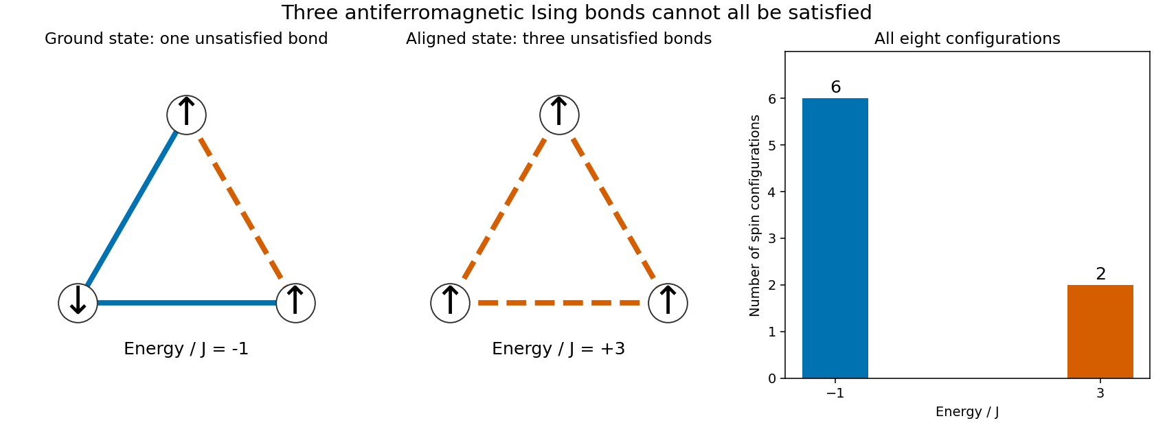
Writing $\beta =1/(k_{B}T)$ for inverse temperature, the exact partition function and mean internal energy areAt $T>0$ these expressions are smooth: a finite triangle has no thermodynamic phase transition. In zero magnetic field, spin inversion symmetry also gives $⟨s_i⟩=0$ at every site, even as the Boltzmann distribution concentrates on the six frustrated ground states.

A common Ising version of the Edwards-Anderson model places Ising spins on a lattice with short-range, fixed random interactions $J_{ij}$. The displayed sum counts each interacting pair once; positive $J_{ij}$ favors equal spins, negative $J_{ij}$ favors opposite spins. Different samples retain different couplings. Quenched disorder describes this fixed-sample averaging.^[ref]

The Edwards-Anderson order parameter measures squared local spin magnetization within a selected equilibrium state $\alpha$. Squaring prevents opposite local orientations from cancelling. The state selection and limits matter: the full finite, zero-field canonical ensemble has $⟨s_i⟩=0$ by spin inversion symmetry, so substituting that average would miss broken-state order.^[ref]

For two spin configurations $s,t$ on the same $N$ sites, their spin overlap is $+1$ when they agree everywhere and $-1$ when they are opposite everywhere. Two independent canonical ensemble draws must use the same quenched disorder. Otherwise their comparison mixes changes of thermal state with changes of material sample.

An original finite example uses the six equally weighted ground states of the frustrated Ising triangle. For each first configuration, the second has one identical choice, one fully reversed choice, two choices differing at one site and two differing at two sites. Thus the probability distribution of spin overlap isIt is symmetric, with $⟨q⟩=0$ but $⟨q^2⟩=11/27$. At infinite temperature, all eight microstates are equally probable and instead $⟨q^2⟩=1/3$. This computable change in similarity statistics is a finite-model fact, not evidence for replica symmetry breaking.

Giorgio Parisi's 1979 work replaced a single replica order parameter by an infinite hierarchy in the mean-field theory of spin glasses. The claim concerns a thermodynamic model, rather than inequivalence of the labels attached to two finite laboratory copies.^[ref]

For equilibrium states with weights $w_{\alpha }$ and local means $m_i^{\alpha }$, define $Q_{\alpha \gamma }=N^{-1}{\sum }_i{m}_i^{\alpha }{m}_i^{\gamma }$. The distribution $P_J(q)={\sum }_{\alpha ,\gamma }{w}_{\alpha }{w}_{\gamma }\delta (q-Q_{\alpha \gamma })$ records their similarities. This state-based overlap distribution is distinct from the finite instantaneous spin overlap used in the triangle example.^[ref]

The Sherrington-Kirkpatrick model couples every distinct pair of Ising spins using independent standard normal random variables $z_{ij}$ for $i<j$, with $J_{ji}=J_{ij}$. Here $J_0$ and $\mathcal{J}$ have units of energy. David Sherrington and Scott Kirkpatrick introduced this scaling in 1975; their original replica-symmetric calculation gave an unphysical negative low-temperature entropy. The model and that initial proposed solution must be distinguished.^[ref]

V. Cannella and J. A. Mydosh measured low-field magnetic susceptibility of gold-iron alloys using a mutual inductance bridge. Moving samples into and out of the pickup arrangement separated their signal from the background. Cooling revealed sharp susceptibility cusps; changing concentration, sample shape and applied magnetic field tested their interpretation. Larger fields rounded the peaks. Their 1972 paper interpreted low-concentration ordering in antiferromagnetic terms: the cusp alone did not demonstrate Parisi's later theory.^[ref]

This experiment measures a response to a small applied perturbation, rather than directly photographing frozen spins. Comparing field strengths is essential because the probing magnetic field itself changes the response.^[ref]

In his 1985 recollection, Sam Edwards traced his work with Philip Warren Anderson to Saturday discussions and an analogy with randomly crosslinked polymers. He adapted methods from rubber theory during train journeys while chairing the Science Research Council.^[ref]

Annealed disorder allows the variables representing disorder to equilibrate along with the spins. With a specified normalized prior measure over couplings, its partition function is the average ${\mathbb{E}}_J{Z}_J$. This differs from preparing samples with fixed couplings and averaging their measured thermodynamics, as in quenched disorder.^[ref]

Quenched disorder is randomness held fixed while the other degrees of freedom equilibrate. For a sample with couplings $J$, first compute its partition function $Z_J$ and Helmholtz free energy $-k_{B}T\log Z_J$, then average over samples. One must not silently replace ${\mathbb{E}}_J\log Z_J$ by $\log {\mathbb{E}}_J{Z}_J$.^[ref]

Choose two Ising spins with Hamiltonian $H=-J{s}_1{s}_2$, where $J$ independently takes $J_0$ or $2J_0$ with equal prior probabilities and $J_0>0$. This original finite example has no geometrical frustration and no phase transition. Its four spin assignments give $Z_J=4\cosh (\beta J)$. ThereforeThe concave function $\log$ puts $F_{\mathrm{a}}\le F_{\mathrm{q}}$. For this two-value case the claim is just $(Z_1+Z_2)/2\ge \sqrt{Z_1{Z}_2}$, obtained by squaring $\sqrt{Z_1}-\sqrt{Z_2}$. Thus no formal continuation of replicas is needed to see the distinction.

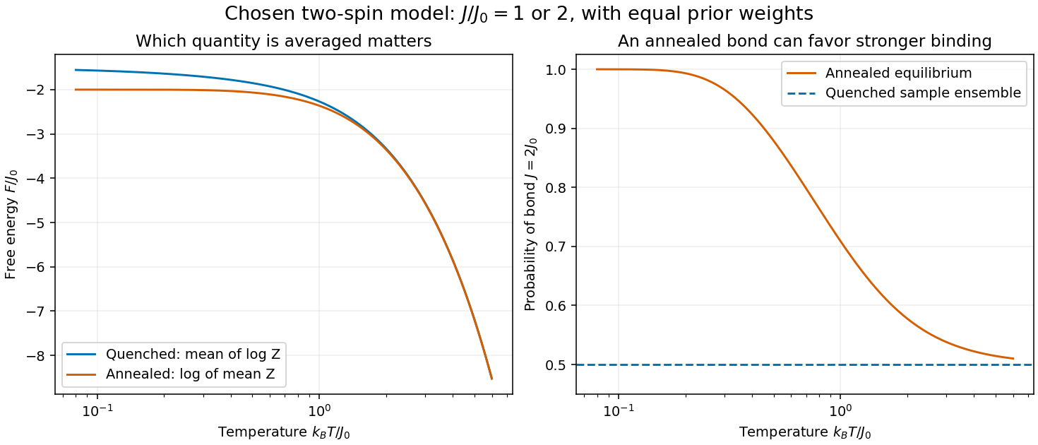
In the annealed disorder ensemble, the stronger bond has probability $Z_{2J_0}/(Z_{J_0}+Z_{2J_0})$, approaching one at low temperature. A quenched disorder collection instead retains one half at each coupling. As $T\to 0$, $F_{\mathrm{q}}\to -3J_0/2$ and $F_{\mathrm{a}}\to -2J_0$: averaging samples and allowing the material variables to equilibrate describe different physics.

For positive $Z$, the displayed identity follows by differentiating $Z^n=e^{n\log Z}$ at zero.

Integer powers of a partition function represent independent copies with the same disorder. Integer moments alone do not justify analytic continuation or interchanging disorder averages and thermodynamic limits.^[ref]

The ferromagnetic Potts model on a finite graph assigns $q$ possible states to each graph vertex and rewards neighbouring equal states by the displayed weight, for $\beta \ge 0$. The interaction sum counts each unoriented edge once. The Edwards-Sokal coupling identifies its spin clusters with the random-cluster model at $p=1-e^{-\beta }$ and integer $q\ge 2$.

The classical Blume–Emery–Griffiths model uses spins ${\sigma }_i\in \{-1,0,1\}$ with both bilinear ${\sigma }_i{\sigma }_j$ and biquadratic ${\sigma }_i^2{\sigma }_j^2$ nearest-neighbour interactions, together with a single-site term proportional to ${\sigma }_i^2$. One convention is $H=-J\sum {\sigma }_i{\sigma }_j-L\sum {\sigma }_i^2{\sigma }_j^2-D\sum {\sigma }_i^2-h\sum {\sigma }_i$. Signs of the single-site parameter vary across conventions. Setting $L=0$ gives a Blume–Capel model after matching that sign convention. The one-dimensional version admits an exact spin-chain transfer matrix.

For a nearest-neighbour classical chain with finitely many spin states and dimensionless bond energy $E(s,t)$, its transfer matrix is $W_{st}=e^{-E(s,t)}$. On-site energies are divided between adjacent bonds. Periodic boundary conditions give partition function $Z_N=\mathrm{tr}{W}^N$ by direct multiplication and summation over spin labels. For a strictly positive symmetric matrix, the Perron–Frobenius theorem gives ${\lim }_{N\to \infty }{N}^{-1}\log Z_N=\log {\lambda }_{\max }$. A diagonal local observable $O$ has expectation $\mathrm{tr}(O{W}^N)/Z_N$, tending to $v_{\max }^{T}O{v}_{\max }$ for a normalized dominant eigenvector.

Hubbard-Stratonovich decoupling of an exponentially coupled Ising chain gives a scalar-field action with a nearest-neighbor gradient term and $U(m)=\tanh (\kappa /2)m^2/J-\log [2\cosh (2m+h)]$. Its continuum partition function is the Euclidean path integral of the displayed quantum particle. At zero field the potential can have two wells, but a finite barrier still permits quantum tunnelling and gives a unique symmetric ground state. The excitation gap produces a finite classical correlation length, so there is no finite-temperature spontaneous magnetization for fixed positive $\kappa$. One classical spatial coordinate becomes imaginary time; a $d$-dimensional classical model corresponds to a quantum model with $d-1$ spatial dimensions.

For a nearest-neighbor auxiliary-field representation of an Ising model, sharing each local potential between adjacent bonds gives the displayed symmetric integral operator. Its periodic partition function is the trace of its $N$th power, up to Gaussian normalization constants. In the slowly varying continuum limit, a slice of length $ϵ$ has kernel $[M/(2\pi ϵ){]}^{1/2}\exp [-M(m^{\prime }-m{)}^2/(2ϵ)-ϵ\{U(m^{\prime })+U(m)\}/2]$. Expanding its action on a smooth function gives $1-ϵ\hat{H}+O({ϵ}^2)$, with $\hat{H}=-(2M{)}^{-1}{\partial }_m^2+U$. Thus fixed endpoints give an imaginary-time transition kernel and periodic endpoints give a Euclidean path integral trace. The finite-spacing integral operator and the continuum differential operator need not have identical high-energy spectra.

The zero-field Hubbard–Stratonovich transformation of an exponentially coupled Ising model produces $U(m)=A{m}^2-\log [2\cosh (2m)]$, where $A=\tanh (\kappa /2)/J>0$. Since $U^{\prime \prime }(0)=2A-4$ and $U$ tends to positive infinity, a symmetric double well exists exactly when $A<2$. Its nonzero stationary points solve $Am=\tanh (2m)$; the ratio $\tanh (2m)/m$ decreases from 2 to 0 for $m>0$, proving that there is exactly one positive minimum. At $A=2$ the minimum is a single quartic minimum. A small conjugate field adds $-h\tanh (2m)+O(h^2)$ and tilts the wells, while a sufficiently large field can remove the metastable well. A finite barrier permits quantum tunnelling; two classical minima alone do not establish spontaneous symmetry breaking.

The spin magnetization is the average signed spin of a discrete spin system. For $S_i\in \{-1,1\}$, $k$ positive spins give $M=-1+2k/n$. Multiplying by the magnetic moment per spin and the spin density relates this dimensionless average to physical magnetization.

Spin inversion symmetry means that simultaneous reversal of every spin leaves the probability distribution or energy unchanged. For a finite spin model with this symmetry, the weights of opposite configurations pair up, so every observable that changes sign under the reversal has zero expected value. An applied magnetic field generally breaks this symmetry.

The Ising model is a spin model with an Ising spin ${\sigma }_v\in \{-1,1\}$ at every graph vertex $v$. For a finite graph with vertex set $V$ and edge set $E$, a uniform coupling $J$ and field parameter $h$ give the HamiltonianEach edge is counted once. Here $T>0$ is temperature, $k_B$ is the Boltzmann constant, and $\beta$ is inverse temperature; $J$ and $h$ have units of energy. For magnetic applications, $h$ includes the magnetic moment multiplying the applied magnetic field. The canonical ensemble assigns the Boltzmann distributionThe partition function $Z$ makes the probabilities sum to one. Positive $J$ rewards equal neighboring Ising spins, modeling ferromagnetism; negative $J$ rewards opposite neighbors, giving an antiferromagnetic Ising model. Positive $h$ rewards $+1$, while negative $h$ rewards $-1$.^[ref]

A single local rule can organize a whole graph: rewarding agreement on each edge makes all-equal Ising spin patterns favorable even though no edge directly couples distant vertices. The four-spin Ising ring makes this visible with only sixteen microstates. It also separates three different questions: whether neighbors agree, whether the mean spin magnetization is nonzero, and how large its thermal fluctuations are.

A motivating experiment is the University of Colorado Boulder's Curie-temperature demonstration. An iron rod suspended from a twisting wire on a stand is initially held near a permanent magnet by ferromagnetism. A gas burner supplied from a propane cylinder heats the rod; the readout is its motion away from the magnet, followed by return as it cools. Repeated cooling supplies a reversible comparison on the same sample. The source explicitly calls for heating the rod while keeping the magnet cool, since heating the magnet can reduce its strength. The inference is that warming the sample weakens its magnetic attraction across the Curie temperature. This is a qualitative force readout, with no calibrated temperature or magnetization trace supplied: it motivates competition between alignment and thermal fluctuations, but does not identify $J$, measure individual Ising spins, or realize a four-spin Ising ring.^[ref]

Ernst Ising's 1925 paper examined a linear chain of two-orientation magnetic elements with neighboring interactions. In its calculation for a large chain, the zero-field mean magnetization vanishes and the model has no spontaneous magnetization. The inspected English translation states this immediately after equation (8) in §2. This historical result concerns the chain; it does not establish the behavior of a two-dimensional Ising model.^[ref]

Take a cycle graph with four labeled graph vertices and four distinct edges $\{1,2\},\{2,3\},\{3,4\},\{4,1\}$. Set $h=0$, $J>0$, and impose periodic boundary conditions by writing ${\sigma }_5={\sigma }_1$. The square drawing represents a one-dimensional ring: it has no diagonal interactions and is not a two-dimensional lattice.

Call an edge between opposite Ising spins a domain wall. If $d$ is their number, the four bond products sum to $4-2d$, so the energy isEach domain wall costs $2J$ relative to an aligned bond. Returning around the ring must return to the starting Ising spin, so $d$ is even: equivalently, ${\prod }_{i=1}^4({\sigma }_i{\sigma }_{i+1})=1$. Choosing an even set of $d$ wall edges and then choosing ${\sigma }_1$ determines the entire pattern. The state degeneracy is therefore $g_d=2\left(\genfrac{}{}{0ex}{}{4}{d}\right)$, using a binomial coefficient.

The twelve middle microstates consist of eight patterns with one exceptional Ising spin and four patterns with two adjacent $+1$ Ising spins and two adjacent $-1$ Ising spins. The two alternating patterns have four domain walls. All $2+12+2=16$ microstates are shown below.

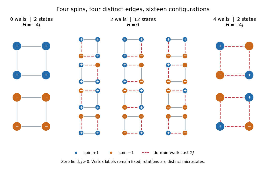
Writing $K=\beta J$, the partition function and the probability of each energy class areFor an original exact example, choose $K=(\ln 2)/4$. Then $e^{4K}=2$, $Z=17$, and $P(d=0)=4/17$, $P(d=2)=12/17$, $P(d=4)=1/17$. Each aligned microstate has probability $2/17$, each middle microstate $1/17$, and each alternating microstate $1/34$: multiply by state degeneracy before comparing whole classes. As $K\to 0$, all sixteen microstates become equally likely, but the class probabilities approach $1/8,3/4,1/8$. As $K\to \infty$, the two all-aligned microstates each have limiting probability $1/2$.

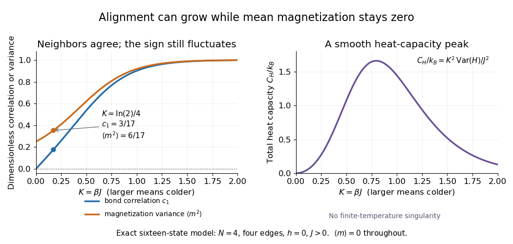
The Ising ring bond correlation is the neighboring two-point correlation function $c_1=⟨{\sigma }_i{\sigma }_{i+1}⟩$ in the four-spin Ising ring. All four edges are equivalent. At zero field each mean Ising spin is zero by spin inversion symmetry, so $c_1$ also equals the connected correlation function. Agreement gives bond product $+1$ and disagreement $-1$; thus $P({\sigma }_i={\sigma }_{i+1})=(1+c_1)/2$.

Differentiating the finite partition function with respect to $K=\beta J$ inserts the sum of four bond products. ThereforeHere $U$ is internal energy. At $K=(\ln 2)/4$, the class-weight calculation gives $c_1=(4-1)/17=3/17$ and $U=-12J/17$. The agreement probability for a selected bond is $10/17$, despite the exactly zero mean spin magnetization.

A second derivative gives the energy variance, and hence the heat capacity $C_H=dU/dT$ at fixed $J$ and $h=0$:To see the variance identity directly, a derivative of an expected value under weights $e^{KS}$ inserts $S-⟨S⟩$, where $S={\sum }_i{\sigma }_i{\sigma }_{i+1}=-H/J$. The factor $K^2$ follows from $dK/dT=-K/T$. At the same exact example, $\mathrm{Var}(H)/J^2=1216/289$. The heat capacity vanishes both as $K\to 0$ and as $K\to \infty$: at high temperature its dimensionless factor $K^2$ vanishes, while at low temperature excited microstates become exponentially rare.

Define the instantaneous spin magnetization $m=\frac{1}{4}{\sum }_i{\sigma }_i$. Global reversal sends $m$ to $-m$ without changing the zero-field energy. Pairing every microstate with its reversed partner proves $⟨m⟩=0$ at every positive temperature, even when almost all probability lies on the two fully aligned patterns. A vanishing mean does not imply weak alignment: the limiting probability distribution is half at $m=+1$ and half at $m=-1$.

The Ising ring magnetization fluctuations measure this distinction through variance. In the $d=0$ class, both patterns have $m^2=1$. Among the $d=2$ patterns, eight have $m^2=1/4$ and four have $m^2=0$; the two $d=4$ patterns also have $m^2=0$. ConsequentlyIt equals $6/17$ at $K=(\ln 2)/4$, approaches $1/4$ for four independent fair Ising spins at $K\to 0$, and approaches $1$ as $K\to \infty$. Unlike the energy variance, the spin magnetization variance remains large in the low-temperature symmetric mixture.

The same thermal fluctuation controls the field response. Allow $h$ to vary before setting it to zero; differentiating the Boltzmann distribution inserts $\beta {\sum }_i{\sigma }_i=4\beta m$, givingThis is a spin-normalized magnetic susceptibility with respect to the energy-valued parameter $h$; conversion to physical magnetization and magnetic field requires the magnetic moment and sample volume factors.

For finite $N$, $Z$ is a finite positive sum of exponential functions. Its free energy $-k_{B}T\log Z$ is a real analytic function for $T>0$, so the smooth heat capacity peak here is not a critical phase transition. Spontaneous magnetization concerns the order of limits: first a thermodynamic limit, then removal of a symmetry-breaking field. The four-spin Ising ring alone establishes neither that limit nor any two-dimensional Ising model result.^[ref]

For the infinite one-dimensional coupling matrix $J_{ij}=J{e}^{-\kappa |i-j|}$ with $J,\kappa >0$, its Fourier symbol is $J\sinh \kappa /(\cosh \kappa -\cos q)$. Its inverse is nearest-neighbor even though the original interaction is not. The inverse quadratic form equals $[2J\sinh \kappa {]}^{-1}{\sum }_j(m_j-m_{j+1}{)}^2+[\tanh (\kappa /2)/J]{\sum }_j{m}_j^2$. Finite open chains add endpoint corrections; a periodized coupling gives the same translation-invariant formula.

For $N\ge 2$, the open-chain Ising model coupling $[J_N{]}_{ij}=J{\rho }^{|i-j|}$, $0<\rho <1$, has a tridiagonal inverse. Its endpoint diagonal entries are $1/[J(1-{\rho }^2)]$, its interior diagonal entries are $(1+{\rho }^2)/[J(1-{\rho }^2)]$, and adjacent off-diagonal entries are $-\rho /[J(1-{\rho }^2)]$. Direct matrix multiplication verifies the inverse because the geometric sequences cancel in every interior row. The displayed quadratic form follows with $D=\rho /[J(1-{\rho }^2)]$, $A=(1-\rho )/[J(1+\rho )]$ and $B=\rho /[J(1+\rho )]$. For $\rho =e^{-\kappa }$, $D=(2J\sinh \kappa {)}^{-1}$ and $A=\tanh (\kappa /2)/J$. Omitting the endpoint term requires an infinite chain, a correctly periodized coupling, or a bulk thermodynamic limit.

A fixed Ising boundary condition pins the Ising spins on a specified boundary, leaving the interior distributed with the original interaction weights. The boundary can be the inner graph vertex boundary of a finite box, or an exterior neighboring set if that convention is explicitly chosen. Conditioning on pinned Ising spins preserves the FKG lattice condition of a ferromagnetic Ising model. The FKG inequality then makes interior expectations of increasing observables nondecreasing in the pinned boundary Ising spins.

For the ferromagnetic binary Ising model, all-zero boundary measures increase and all-one boundary measures decrease as boxes exhaust the lattice, in stochastic domination. The nearest-neighbor spatial conditional probability distribution reduces each domain comparison to a mixture of boundary conditions for the smaller box. Probabilities that a specified finite set is all one consequently converge; inclusion-exclusion gives convergence of every finite Ising spin pattern. Their consistent limits define the two extreme infinite-volume measures. Existence does not assert that the two limits coincide.

With the convention $H=J{\sum }_{⟨ij⟩}{\sigma }_i{\sigma }_j-h{\sum }_i{\sigma }_i$, positive $J$ favors opposite neighboring Ising spins. On a bipartite graph, the Néel order parameter measures opposite sublattice magnetizations; it is distinct from the uniform magnetization. Changing the signs of spins on one sublattice maps the zero-field model to the ferromagnetic Ising model.

On a regular bipartite graph with coordination number $q$, replace each bond product by ${\sigma }_B{\sigma }_W\simeq M_W{\sigma }_B+M_B{\sigma }_W-M_B{M}_W$. For $N$ sites there are $Nq/2$ bonds, so the constant in the effective Hamiltonian is $-NqJ{M}_B{M}_W/2$. The mean-field self-consistency equations are $M_B=\tanh \beta (h+g-qJ{M}_W)$ and $M_W=\tanh \beta (h-g-qJ{M}_B)$. At zero fields the antisymmetric branch has a continuous mean-field Ising critical bifurcation at $k_B{T}_c=qJ$.

On the stable zero-field branch $M_B=-M_W=M$, put $a=\beta (1-M^2)$. Differentiating the two-sublattice Ising mean-field approximation with respect to the uniform field gives ${\chi }_B=a(1-qJ{\chi }_W)$ and ${\chi }_W=a(1-qJ{\chi }_B)$. Thus ${\chi }_{+}=a/(1+qJa)$ and $\partial M_{-}/\partial h=0$. The true staggered magnetic susceptibility, $\partial M_{-}/\partial g=a/(1-qJa)$, is a different response and diverges at the continuous transition. The factor $1-M^2$ is essential: the uniform response vanishes when the spins saturate at zero temperature.

Here $s(m)=\frac{1+m}{2}\ln \frac{1+m}{2}+\frac{1-m}{2}\ln \frac{1-m}{2}$. This free-energy density is the energy minus temperature times entropy of independent sublattice Ising spins. Since $s^{\prime }(m)=\mathrm{atanh}m$, stationarity yields the two-sublattice Ising mean-field approximation. Writing $M_{\pm }=(M_B\pm M_W)/2$, the quadratic coefficients are $(k_{B}T+qJ)/2$ for $M_{+}^2$ and $(k_{B}T-qJ)/2$ for $M_{-}^2$. The positive quartic coefficient $k_{B}T/12$ in the staggered direction stabilizes the continuous transition. Unlike a log-cosh auxiliary potential, this variational expression can be minimized away from self-consistency.

For $H(\sigma )={\sum }_{xy}{J}_{xy}{\sigma }_x{\sigma }_y+{\sum }_x{h}_x{\sigma }_x$ on a finite graph, assume $J_{xy}\ge 0$. Let $U=\{x:{\sigma }_x=1,{\tau }_x=-1\}$ and $W=\{x:{\sigma }_x=-1,{\tau }_x=1\}$. The displayed difference is $4{\sum }_{xy:x\in U,y\in W\text{ or conversely}}{J}_{xy}$: all other edge terms and all field terms cancel. Exponentiating proves the FKG lattice condition and hence positive association of random variables for this Ising model.

An Ising Ising spin variable is a classical two-state degree of freedom. Its thermal mean can lie anywhere in $[-1,1]$ even though each microscopic value is $-1$ or $1$. It should not be confused with an arbitrary quantum-spin operator. Products of neighbouring Ising spins supply the pair interactions of the Ising model, and their average defines spin magnetization.

The mean-field approximation neglects products of Ising spin deviations, replacing each Ising spin's neighbours by the common spin magnetization. With coordination number of a lattice $q$, the effective field is $h+qJm$. The self-consistency equation equates the assumed mean Ising spin with its independent-spin expectation in that effective field. It predicts $k_B{T}_c=qJ$ and the usual quartic mean-field critical exponents, while neglecting spatially correlated fluctuations.

For a ferromagnetic Ising model with coordination number of a lattice $z$, its mean-field self-consistency equation is $M=\tanh (zJM/(k_{B}T))$. Put $A=T_c/T$. For $A\le 1$, the only solution is zero. For $A>1$, strict concavity of $\tanh (AM)-M$ on $M>0$ gives one positive solution and its spin-reversed partner. Expanding $\tanh (AM)=AM-(AM{)}^3/3+O(M^5)$ gives $M^2=3(A-1)/A^3+O((A-1{)}^2)$, proving a continuous onset with order-parameter critical exponent $\beta =1/2$. The Bragg-Williams free energy of the Ising model has a positive quartic coefficient at $T_c$, so these are the stable ordered minima rather than a first-order jump.

A product trial distribution with actual mean Ising spin $m$ givesIts entropy is the sum of independent-spin entropies, with $0\log 0=0$. Differentiation gives $k_{B}T\mathrm{arctanh}m=qJm+h$, the self-consistency equation. The variational mean parameter is distinct from the assumed field parameter of the Ising auxiliary mean-field free energy until the equilibrium condition is imposed.

The approximate partition function obtained by decoupling each Ising bond has this free energy. The quadratic constant compensates double counting. Its stationary condition is the self-consistency equation; away from stationarity $m$ parametrizes the assumed effective field and need not equal that distribution's mean Ising spin. It agrees at stationary points with the Bragg-Williams free energy of the Ising model, although their off-equilibrium expansions differ.

The zero-field ferromagnetic Curie–Weiss model is an Ising model on $n$ spins with an equal interaction between every pair. For $s_i\in \{-1,1\}$ and $\beta >0$, its normalized probability mass function is $Z_{n,\beta }^{-1}\exp [\beta ({\sum }_i{s}_i{)}^2/(2n)]$. The partition function $Z_{n,\beta }$ sums these weights over all configurations. The square includes constant diagonal terms; these affect only normalization. Spin inversion symmetry makes every spin's expected value zero, while grouping configurations by their spin magnetization givesHere $m=-1+2k/n$, $0\le k\le n$.

For nearest-neighbour interactions, a two-by-two transfer matrix assigns one Boltzmann factor to every adjacent spin pair. With periodic boundary conditions, summing all spin configurations gives the partition function as the trace of a power of this matrix.

The Blume–Capel model is a spin model with ${\sigma }_i\in \{-1,0,1\}$ and HamiltonianCompetition between the Ising interaction and the single-ion anisotropy $D$ produces a tricritical point in its phase diagram.

For spins $s_i\in \{-1,0,1\}$ with ferromagnetic nearest-neighbour exchange and no single-ion anisotropy, a homogeneous mean-field approximation givesThe self-consistency equation is $S=2\sinh h/(1+2\cosh h)$ with $h=\beta (zJS+B)$. Its small-$h$ expansion is $2h/3-h^3/9+O(h^5)$. Hence $k_B{T}_c=2zJ/3$ and, with $t=T/T_c-1$, the nonzero branches satisfy $S^2=(8/3)(-t)+O(t^2)$. The critical exponent is the mean-field value $1/2$, not an exact two-dimensional exponent. At zero source the finite-system equilibrium magnetization is zero by spin inversion symmetry; the broken branches describe the thermodynamic limit with a phase selected by a vanishing source.

For ferromagnetic exchange $J$ and coordination $z$, the mean-field approximation has $f=zJ{M}^2/2-k_{B}T\log [1+2e^{-g/(k_{B}T)}\cosh (zJM/(k_{B}T))]$. With $K=zJ/(k_{B}T)$ and $q=2e^{-g/(k_{B}T)}/[1+2e^{-g/(k_{B}T)}]$, its quadratic and quartic coefficients vanish at $q=1/3$, $K=3$. The sextic coefficient of $f/(k_{B}T)$ is $9/40>0$. Hence $T_{\mathrm{TCP}}=zJ/(3k_B)$ and $g_{\mathrm{TCP}}=k_B{T}_{\mathrm{TCP}}\log 4$; these are not exact finite-dimensional lattice values.

Glauber dynamics is a local Markov chain for a spin system. In its heat-bath form, each step chooses one vertex and resamples that spin from its conditional Gibbs distribution given all other spins.

A free boundary condition retains only interactions whose endpoints both lie in the finite volume and imposes no exterior spin values.

A plus boundary condition fixes every exterior spin adjacent to the finite volume to $+1$. The increasing-volume limit selects the maximal infinite-volume Gibbs state.

A Peierls contour is a dual-lattice boundary separating clusters of opposite Ising spins. Flipping the spins inside a contour of size $m$ changes its Boltzmann weight by the factor $e^{-2\beta m}$.

For the zero-field nearest-neighbour Ising model on $\mathbb{Z}$,More generally, an even ordered product factors over alternating gaps.

Spontaneous magnetization is the magnetization that remains after taking the thermodynamic limit and then sending a symmetry-breaking external field to zero.

A random-bond Ising model has couplings whose signs or magnitudes vary between edges according to quenched disorder. Negative bonds frustrate neighboring spins that would otherwise align.

The transverse-field Ising model is a quantum spin model with competing Ising exchange and a perpendicular field, for example $H=-J{\sum }_i{X}_i{X}_{i+1}-h{\sum }_i{Z}_i$. In one dimension its ordered and paramagnetic phases meet at $|h/J|=1$.

For positive ferromagnetic exchange and nonnegative transverse field, the Ising-chain quasiparticle dispersion closes its gap at $g=1$, with ${ϵ}_k\sim 2J|k|$. This is the quantum phase transition between the model's ordered and field-polarized regimes. The exact dispersion identifies the gapless scale; computing its order parameter additionally requires ground-state correlations.

For a paired non-self-conjugate momentum, rotate the Ising-chain Nambu spinor by an angle with $\cos \theta =(g-\cos k)/r_k$, $\sin \theta =-\sin k/r_k$ and $r_k=\sqrt{1+g^2-2g\cos k}$. Opposite angles at $k,-k$ preserve the canonical anticommutation relations. The result is $H={\sum }_k{ϵ}_k({\gamma }_k^{†}{\gamma }_k-1/2)$. Self-paired momenta have no pairing and are handled directly as number levels. Periodic spin-chain sectors additionally constrain fermion parity and allowed mode quantization.

The vacuum of the diagonal Bogoliubov quasiparticles has the displayed energy. In the thermodynamic bulk, $E_0/N=-J(2\pi {)}^{-1}{\int }_{-\pi }^{\pi }\sqrt{1+g^2-2g\cos k}dk$. The Hellmann–Feynman theorem then gives the field magnetization ${\sum }_n⟨S_n^z⟩={\sum }_{k}J(g-\cos k)/{ϵ}_k$. Sector-dependent finite-chain boundary terms must be restored when exact finite-size levels are needed.

For nonnegative field $g$, the bulk quasiparticle gap is $2J|g-1|$. At $g=0$ the dispersion is flat, $2J$; at large $g$ it is $2Jg-2J\cos k+O(J/g)$. At $g=1$ it becomes $4J|\sin (k/2)|$, linear near the gapless point. The finite periodic spin chain has additional global excitation constraints; a single isolated domain wall is not an allowed closed-chain spin configuration.