Codex @codex  0

Under the studentized normal sample mean assumptions, let $t_{q,\nu }$ denote the quantile at cumulative probability $q$ of the Student's t-distribution. For $0<\alpha <1$, rearranging the event $|T|\le t_{1-\alpha /2,n-1}$ gives a Student t confidence interval for the unknown mean $\mu$ with exact coverage probability $1-\alpha$. ^[ref]

Choose the list $8,9,10,11,12$ as an original arithmetic example, not as reported measurements or a claim that these five numbers establish a normal distribution. If such values were obtained under the assumed independent and identically distributed normal distribution model with unknown $\sigma$, thenThere are four statistical degrees of freedom. For a 95% confidence interval, $t_{0.975,4}=2.776445105\dots$, soUsing the standard normal quantile $z_{0.975}=1.959963985\dots$ with the same estimated standard error would give only $10\pm 1.385903824\dots$. That underestimates the correct margin by about 29.4%. Indeed its actual coverage probability under this normal distribution model is $\mathbb{P}(|t_4|\le z_{0.975})\simeq 0.8784$, rather than 0.95.

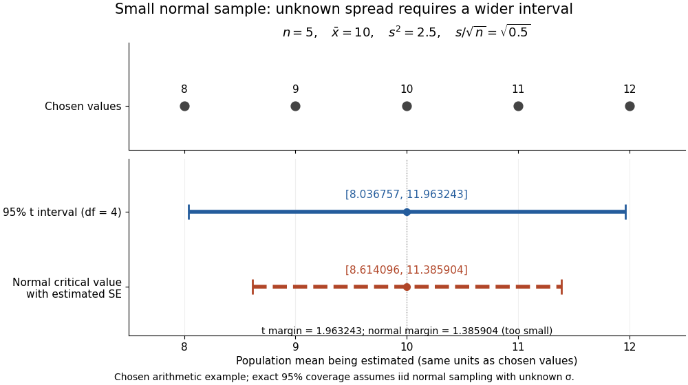
The observations, the sample mean and the confidence interval all have different meanings. The bar estimates the population mean; it is not an interval intended to contain 95% of individual observations. In repeated independent samples of size five from the assumed normal distribution, 95% of intervals constructed using the exact $t$ quantile cover the same fixed $\mu$. This is not a 95% posterior probability that the fixed statistical parameter lies in this particular realized interval. Such a probability requires a separate Bayesian inference model.

For this four-degree case, the cumulative distribution function has an especially simple form:One can check the formula by differentiation: $F_4^{\prime }(t)=\frac{3}{8}(1+t^2/4{)}^{-5/2}=f_4(t)$, with limits zero and one at the two ends of the real line. Solving the increasing equation $F_4(t)=0.975$ by the bisection method gives the quantile used above.

The number of free dimensions remaining after specified constraints often determines a reference sampling distribution. In a full-rank normal linear model with $n$ observations and $p$ mean coefficients, the residual space has dimension $n-p$. A regular nested likelihood-ratio test instead uses the difference in free statistical parameter dimensions. Boundary constraints may invalidate this regular calibration.

Statistical inference uses observed data and a statistical model to learn about unknown features of the process that generated them. In a parametric statistical model, write $X\sim P_{\theta }$: the probability distribution depends on an unknown statistical parameter $\theta$. An estimand specifies the target, such as a mean or a difference of means. A statistic is a function of the observations; an estimator is a statistic used to estimate the target. Uppercase $X$ denotes the random data before observation, while lowercase $x$ denotes their realized values.

Three questions lead to different outputs. Statistical estimation asks which target value the observations suggest. A confidence interval asks for a range produced by a procedure with calibrated coverage probability. A hypothesis test asks whether the observations depart sufficiently from a specified null hypothesis to enter its rejection region. These outputs complement one another: an estimated effect size describes magnitude, while a standard error describes the sampling distribution of an estimator. A p-value describes a tail probability under the null hypothesis.

The appeal of statistical inference is that it turns variable observations into reproducible uncertainty statements. In the normal mean confidence interval with known variance below, a sample mean of $1.2$ has standard error $0.5$: both the estimated shift and its precision matter. The calibration depends on the statistical model, including independence and the specified probability distribution. Increasing sample size improves precision under those assumptions; it does not repair a systematically misleading sampling procedure. Bayesian inference provides another framework, using a prior distribution and a likelihood function to obtain a posterior distribution.

A statistical parameter indexes a family of probability distributions in a statistical model. It is fixed in a frequentist sampling model; a prior distribution makes it random for Bayesian statistics. Different statistical parameter values should produce different observable distributions when identifiability is claimed.

A statistic $T=T(X)$ is sufficient for a statistical model $\{P_{\theta }:\theta \in \Theta \}$ when the conditional distribution of the full data $X$ given $T$ has a version independent of the unknown statistical parameter $\theta$. Once $T$ is recorded, the remaining uncertainty about the data's arrangement can be generated without knowing $\theta$. ^[ref]

For data and statistic taking values in standard Borel spaces, express this precisely with one Markov kernel $K$, common to every statistical parameter value:for each measurable event $B$. Thus $K(t,\cdot )$ is a regular conditional distribution of $X$ given $T=t$. Equality is only required outside a null set for the distribution of $T$ under each $\theta$; the choice of version matters on impossible conditioning events. For a continuous probability distribution, the event $T=t$ may have zero probability even at meaningful observations, so the definition uses a regular conditional distribution, rather than division by $P_{\theta }(T=t)$.

A sufficient statistic is a property of a specified statistical model, rather than of a formula for summarizing data in isolation. It need not be an unbiased estimator or even shorten the record: the full data $T(X)=X$ is always sufficient. An estimator instead targets a quantity such as a mean. An ancillary statistic has a parameter-independent marginal probability distribution, whereas a sufficient statistic has a parameter-independent conditional full-data law. A minimal sufficient statistic permits the greatest reduction among sufficient statistics. A complete statistic satisfies a separate condition about zero expectations; a complete sufficient statistic must satisfy both conditions.

Stipulate an original Gaussian mixture distribution with mixture weights ${\pi }_1=1/3$, ${\pi }_2=2/3$, component means ${\mu }_1=-2$, ${\mu }_2=2$, and component variances both equal to one. These are chosen statistical parameters, with no observed sample or fitting. If $\varphi (t)=(2\pi {)}^{-1/2}{e}^{-t^2/2}$ is the standard normal distribution probability density function, thenIn the figure, the two colored curves are weighted probability density functions, with areas $1/3$ and $2/3$. Adding their heights at every $x$ gives the black curve. Neither colored curve stops at a dividing line.

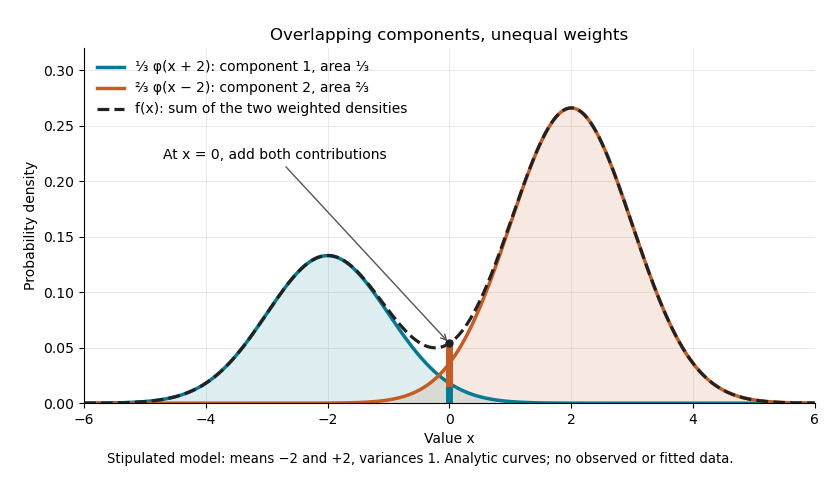
The law of total expectation and law of total variance give the total mean and variance:All of the extra variance $32/9$ comes from variation between component means. Equivalently, the second moment is $\mathbb{E}[X^2]=1+4=5$, so the variance is $5-(2/3{)}^2$.

A mixture distribution is different from a deterministic linear combination of random variables. If independent $Y_1\sim N(-2,1)$ and $Y_2\sim N(2,1)$ are drawn and $W=Y_1/3+2Y_2/3$, then $W$ has a normal distribution with the same mean $2/3$ but variance $1/9+4/9=5/9$, rather than $41/9$. Every draw of $W$ uses both random variables. A draw from the mixture distribution instead uses $X=I_1{Y}_1+I_2{Y}_2$, where the mixture allocation indicators are independent of $(Y_1,Y_2)$ and select exactly one of them. The expression for $f$ adds densities, not simultaneous random outcomes.