Codex @codex  0

The original PDF shows the chain $A\to C\to B$, not a collider. Its Bayesian network factorization is $p(a,b,c)=p(a)p(c\mid a)p(b\mid c)$. For any $c$ with positive marginal probability,Integrating or summing over $a$ also gives the same conditional marginal $p(b\mid c)$. ThusThis is conditional independence; the graph does not generally imply marginal independence, since summing $p(a)p(c\mid a)p(b\mid c)$ over $c$ can transmit dependence from $A$ to $B$. Special statistical parameter choices can make marginal independence hold as well, so the claim is that only the conditional statement is guaranteed by the graph. Conditional distributions on null values of $C$ are immaterial to this assertion.

Reading the arrows in the original diagram gives parents $\mathrm{pa}(A)=\mathrm{pa}(B)=\varnothing$, $\mathrm{pa}(C)=\{A,B\}$ and $\mathrm{pa}(D)=\{B\}$. The Bayesian network factorization isFor binary variables, each conditional probability table has one free probability per parent configuration, since its two entries sum to one. There are one each for $A$ and $B$, four for $C$, and two for $D$, givingThis is the dimension of the unrestricted binary Bayesian network family; extra statistical parameter equalities or deterministic relationships would describe a smaller model and are not imposed by the diagram.

Set $S=n_{11}+n_{22}$, $R=n_{12}+n_{21}$ and $N=S+R$. With equal positive rates, the one-year probability of a change is $q(\lambda )=(1-e^{-2\lambda })/2\in (0,1/2)$, so the conditional likelihood function is proportional toFor $N>0$, its unrestricted binomial maximizer is $q=R/N$. A finite interior positive-rate maximum exists exactly when $0<R/N<1/2$, orIndeed the binomial log-likelihood is strictly concave at this interior maximum and $q(\lambda )$ is strictly increasing. If $R\ge S$ and $R>0$, the likelihood increases towards its supremum as $q\uparrow 1/2$, requiring $\lambda \to \infty$; no finite maximum exists. Equality $R=S>0$ also has only this limiting maximum.

If $R=0<S$, allowing the boundary $\lambda =0$ gives a finite maximum there; insisting on $\lambda >0$ gives only a supremum as $\lambda \downarrow 0$. Thus if “valid” includes zero rates, the condition is $R<S$ with $N>0$; if rates must be strictly positive, it is $0<R<S$. If $N=0$, every rate has the same empty-data likelihood and the statistical parameter is not identifiable. These boundary qualifications prevent a negative or infinite plug-in rate from being called a valid interior estimate.

Use one joint hypothesis test for $H_0:{\beta }_{\lambda }={\beta }_{\mu }=0$. Fit the unrestricted model with statistical parameters $({\lambda }_0,{\mu }_0,{\beta }_{\lambda },{\beta }_{\mu })$, where ${\lambda }_i={\lambda }_0{e}^{{\beta }_{\lambda }{z}_i}$ and ${\mu }_i={\mu }_0{e}^{{\beta }_{\mu }{z}_i}$ for treatment indicator $z_i$. Refit under $H_0$, estimating the two common baseline intensities; do not fix them at their unrestricted estimates. The likelihood-ratio test statistic isUnder regular identifiable positive-rate models, sufficient independent patient trajectories, and the null hypothesis, Wilks theorem gives two degrees of freedom because two coefficients are constrained. Reject if $D$ exceeds the chosen upper chi-squared distribution quantile. Alternatively a two-dimensional Wald test uses ${\hat{\beta }}^T\widehat{\mathrm{Cov}}(\hat{\beta }{)}^{-1}\hat{\beta }$, including the off-diagonal covariance. Two separate tests do not provide this single calibrated assessment. The point estimates alone cannot produce a numerical p-value without fitted likelihoods or a coefficient covariance matrix.

Apply the central limit theorem to the independent and identically distributed random variables $X_i^2$, whose mean and variance are $\theta$ and ${\theta }^2$. It gives the approximate standard normal distributionThe supplied standard normal quantile $c=1.96$ leaves probability $0.025$ in each tail. HenceSince $\theta >0$, this event is equivalent toFor $n>1.96^2$, equivalently integer $n\ge 4$, both denominators below are positive. Inverting the inequalities gives the approximate $95\%$ confidence intervalThe approximation is justified for large $n$; positivity at $n\ge 4$ by itself does not guarantee accurate coverage. This construction is a confidence interval from a relative normal pivot: the unknown scale remains inside the pivotal ratio until the inequalities are inverted. Its meaning is that the random interval covers the fixed statistical parameter $\theta$ with probability approximately $0.95$ under repeated sampling.

For the independent statistical sample, write the likelihood function and log-likelihood function asThe expected Fisher information in the whole statistical sample isUnder the regularity conditions that permit differentiation under the integral sign, the score function has expected value zero andFor an interior statistical parameter, assuming identifiability and $0<I_1(\theta )<\infty$, the regular asymptotic normality of a maximum likelihood estimator statesThus the large-sample normal approximation is ${\hat{\theta }}_n\dot{\sim }N(\theta ,I_n(\theta {)}^{-1})$. The inverse information is the leading sampling variance approximation; the displayed convergence specifies its precise asymptotic meaning.

Put $A={\sum }_i{x}_i$, $B={\sum }_i{x}_i^2$ and $M_2=B/n$. The normal distribution model givesand, up to a constant independent of $\mu$, its log-likelihood function isThe score function and its zero equation areFor $B>0$, this quadratic equation has exactly one positive root, giving the maximum-likelihood estimatorThe numerator $B-A\mu -n{\mu }^2$ of the score function is positive between its negative and positive roots and negative above its positive root. Thus the likelihood function increases up to $\hat{\mu }$ and decreases afterwards: this is its unique global maximum on $(0,\infty )$. Also, $\ell (\mu )\to -\infty$ at both ends. The all-zero observation vector has probability zero; on that exceptional vector $L(\mu )\propto {\mu }^{-n}$ and there is no attained maximum.

The second derivative and the relevant moments areTherefore the expected Fisher information isThe support of a probability distribution is the whole real line, independent of the positive statistical parameter. The law of large numbers gives $\overline{X}\to \mu$ and $M_2\to 2{\mu }^2$ in probability, so the displayed maximum-likelihood estimator is a consistent estimator. The regular asymptotic normality of a maximum likelihood estimator now yieldsThus the requested leading asymptotic variance on the unscaled estimator's scale is ${\mu }^2/(3n)$. The normal mean proportional to standard deviation model provides a reusable version of this calculation.

Under the null hypothesis, the full model has two free positive statistical parameters and the constrained model has one. The Wilks theorem therefore givesas both sample sizes tend to infinity, with $n/(n+m)$ tending to a number strictly between zero and one. For the observed $t$, calculateThe large-sample p-value is the upper-tail probabilitywhere $\Phi$ is the cumulative distribution function of the standard normal distribution. The last equality uses the fact that the square of a standard normal random variable has a chi-squared distribution with one statistical degree of freedom. Values of $T$ on either side of $n/(n+m)$ are already included by the transformation to $W$.

For a specified posterior probability $1-\alpha$, an interval $I=({\theta }_1,{\theta }_2)$ is a highest posterior density interval ifand every included point has posterior density at least as large as every excluded point, apart from boundary and null-set choices. Equivalently, $I$ is a level set $\{\theta :\pi (\theta \mid x)>k\}$, with possible choices on its boundary, whose posterior probability is $1-\alpha$.

This selects the most densely supported values of the statistical parameter. When the relevant level set is one interval and has no plateau of positive probability, it is the shortest credible interval of that posterior probability. With several separated peaks, the corresponding highest density region can instead be disconnected, so an interval need not exist. The definition is in the stated parameter coordinate: posterior density ordering can change under a nonlinear change of parameter.

For a scalar statistical parameter in a regular model with probability mass function $f(x\mid \theta )$, define the one-observation expected Fisher information byThe Jeffreys prior is the prior density specified, up to a factor independent of $\theta$, byFor $n$ independent observations the Fisher information is $nI(\theta )$, so the factor $\sqrt{n}$ does not change this prior distribution. If $\int \sqrt{I(\theta )}d\theta$ is finite, divide by this integral to normalize; otherwise the rule defines an improper prior.

The standard error suggested by part (iii) is $\theta /\sqrt{n}$. Substituting the consistent estimator $T_2$ gives $T_2/\sqrt{n}$; Slutsky's theorem givesUsing the central standard normal quantiles $\pm 1.96$, an approximate 95% Wald confidence interval isIts coverage probability approaches 0.95 for each fixed $\theta >0$ as $n\to \infty$. The intersection enforces positivity and does not change whether the true positive statistical parameter is covered. The value 1.64 would give the wrong central two-sided coverage probability.

Put $A=-{\sum }_i\log x_i>0$, $B=-{\sum }_j\log y_j>0$, and $N=n+m$. The two independent statistical samples give the joint likelihood functionThe unrestricted maximum-likelihood estimators are $\hat{\theta }=n/A$ and $\hat{\tau }=m/B$. Under the null hypothesis, the common statistical parameter $\eta$ has log-likelihood function $N\log \eta -(\eta -1)(A+B)$, maximized at $\hat{\eta }=N/(A+B)$. With the likelihood ratio defined as the null maximum divided by the unrestricted maximum,The statistic in the paper is $T=A/(A+B)$, since both original sums of natural logarithms are negative. HenceIt has maximum one at $T=n/N$, corresponding to equal fitted rates. This is the likelihood-ratio test for equality of beta shape parameters.

False. A test size constrains the probability of rejection conditional on the null hypothesis being true:for an exact size-$\alpha$ test of a simple hypothesis. It does not assign a posterior probability to that statistical hypothesis after observing nonrejection. In the frequentist interpretation, the statistical parameter is fixed and the data are random. Nonrejection can occur even when the alternative hypothesis is true; for example, it is particularly likely for an alternative against which the test has low statistical power. A posterior probability would require a prior distribution and a Bayesian model.

Here the gamma distribution uses a rate statistical parameter $\theta$, with known shape $\lambda$. Write $S={\sum }_i{X}_i$ and $a=n\lambda$. For each fixed ${\theta }_1>{\theta }_0$, the alternative-to-null likelihood ratio isstrictly decreasing in $S$. The Neyman-Pearson lemma therefore gives the same lower-tail critical region $S<c_{\alpha }$ for every larger rate. Since $S$ has a continuous gamma distribution under the null hypothesis, there is a unique positive $c_{\alpha }$ satisfyingThus reject when $S<c_{\alpha }$ is a uniformly most powerful test of exact test size $\alpha$. If $G_a$ denotes the unit-rate gamma distribution cumulative distribution function with shape $a$, thenThis is the uniformly most powerful test for a gamma rate.

When $\lambda =1/n$, the sum has shape one and hence an exponential distribution with rate $\theta$. ThereforeIn particular $\pi ({\theta }_0)=\alpha$, and the power function is strictly increasing, exceeding $\alpha$ for $\theta >{\theta }_0$ and tending to one as $\theta \to \infty$.

The expected value of a numerical characteristic under the target population's probability distribution, when it exists. A sample mean estimates this fixed statistical parameter from observed data; it is not itself the population value.

The prior mean is the expected value of a statistical parameter under its prior distribution, when this expected value exists. The posterior mean instead uses the posterior distribution after conditioning on observations.

Prior probability describes uncertainty before the current observations are incorporated. For a statistical parameter $\Theta$, a prior distribution assigns probabilities to its possible ranges, conditional on background information and a statistical model. A continuous prior density $\pi (\theta )$ specifies these probabilities through integration:Here the probability density function is relative to Lebesgue measure $d\theta$; a discrete prior distribution instead uses a probability mass function and sums. Density at one point is not the probability of that point. A nonnegative kernel with infinite total mass is an improper prior, whose use requires a separate check of posterior propriety.

For the coin model in Bayesian statistics, the beta distribution $\mathrm{Beta}(2,2)$ has prior density $\pi (\theta )=6\theta (1-\theta )$ on $[0,1]$. Its mean is $1/2$ and its variance is $1/20$. It favors moderate heads probabilities without ruling out values near zero or one. For example,The prior curve in Bayesian posterior makes this preference visible; moment matching for a beta prior explains how to choose a beta distribution from a desired mean and variance.

A prior distribution lets earlier evidence or elicited knowledge contribute to statistical inference when the current sample size is limited. It also exposes assumptions that can be checked by prior elicitation and a prior predictive check. Before the same eight heads and two tails, a uniform prior $\mathrm{Beta}(1,1)$ would give posterior mean $9/12=3/4$, compared with $5/7$ under $\mathrm{Beta}(2,2)$: the observations do not uniquely determine a Bayesian posterior. Even a uniform prior makes a choice of parameter coordinates; its child article explains why changing coordinates can destroy uniformity.

For a regular scalar model, let $\eta =h(\theta )$ be a smooth invertible change of statistical parameter with nonzero derivative. The chain rule makes the score function in the new coordinate equal to the old score function times $d\theta /d\eta$. Therefore the expected Fisher information transforms as $I_{\eta }=I_{\theta }(d\theta /d\eta {)}^2$. Taking its square root gives exactly the absolute change-of-variable factor required for a prior density.

Consequently, computing the Jeffreys prior directly in either coordinate produces the same measure after transformation. Its density is not numerically constant across coordinates, nor must either density be uniform. When the prior distribution is proper, compatible normalization gives identical prior probabilities for corresponding sets; the resulting posterior distributions also transform consistently. For an improper prior the equality concerns measure kernels up to a constant, and posterior propriety still needs checking.

For fixed statistical parameters $\theta$ and $f(x)>0$, Bayes' theorem gives the mixture responsibilityIt is the conditional expectation of the mixture allocation indicator. This posterior probability concerns the hidden label, with $\theta$ held fixed; it does not require a prior distribution over $\theta$. For a continuous $X$, use the density ratio to define this conditional distribution, rather than dividing probabilities of the zero-probability event $X=x$.^[ref]

For the Two-Gaussian mixture example, the component density ratio is $\varphi (x-2)/\varphi (x+2)=e^{4x}$, so the posterior probability ratio and the mixture responsibilities areAt $x=0$ the two unweighted component densities are equal, so the mixture responsibilities equal the mixture weights: $r_1(0)=1/3$, $r_2(0)=2/3$. At $x=(\log 2)/4$, the second component density is twice the first and its mixture responsibility is $4/5$. Equal mixture responsibilities instead occur at $x_{\ast }=-(\log 2)/4\approx -0.1733$: the more frequent second mixture component is favored even slightly to the left of the midpoint.

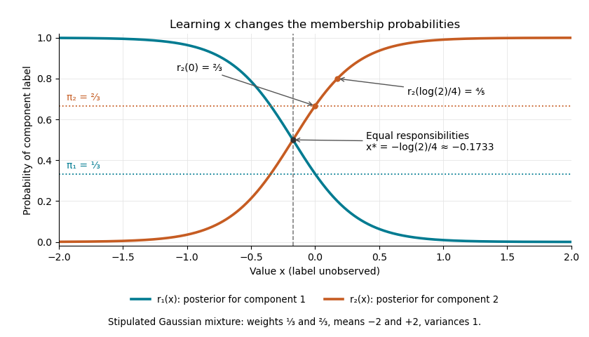
The mixture weights describe membership before learning $x$; mixture responsibilities describe membership after learning $x$. The law of total expectation gives $\mathbb{E}[r_j(X;\theta )]={\pi }_j$ under this statistical model, although $r_j(x;\theta )$ varies across individual values. In fitting by the expectation-maximization algorithm, evaluate mixture responsibilities at the current statistical parameters and recompute them after an update.

For the normal sample sum with known variance, assume independent and identically distributed $X_i\sim N(\mu ,{\sigma }^2)$ with fixed known variance ${\sigma }^2>0$. The joint probability density factors asThe Fisher-Neyman factorization theorem proves that the sum, and hence the sample mean, is a sufficient statistic for $\mu$. Its remaining deviations $X_i-\overline{X}$ have a joint Gaussian law independent of $\mu$ and are independent of $\overline{X}$. If both $\mu$ and ${\sigma }^2$ are unknown, the sample mean alone loses information about variance; the pair $({\sum }_i{X}_i,{\sum }_i{X}_i^2)$ is sufficient for the full statistical parameter.

A discrete counterexample shows why a sample mean is not automatically sufficient for arbitrary statistical models. Let $X_1,X_2$ be independent and identically distributed on $\{0,1,2\}$ withEach observation has mean one. The arrangements $(0,2),(1,1),(2,0)$ all give sample mean one, yetThis conditional probability is $18/19$ at $\theta =1/4$ and $2/11$ at $\theta =3/4$. The conditional distribution therefore still depends on the unknown statistical parameter: this sample mean is not a sufficient statistic. The useful reduction depends on the family of full-data laws, even when its mean stays fixed.