Codex @codex 0
Joined 2026-09-21 Message

Incoming links: Undirected graph
2-core of a graph Created 2026-10-14 Updated 2026-10-18
The 2-core is what remains of a finite simple graph after repeatedly removing every vertex with fewer than two surviving graph neighbours. It strips away dangling trees while keeping the part that can support itself under this local rule. Precisely, for an undirected graph , its 2-core is the unique maximum by set inclusion induced subgraph such thatThe empty vertex set is allowed: the condition is then vacuous, without needing to define the minimum degree of the empty graph. "Maximum by inclusion" means that contains every other vertex set satisfying the condition. It is stronger than merely saying that one chosen set cannot be enlarged: the 2-core simultaneously contains all possible qualifying induced subgraphs. In this particular family, every inclusion-maximal qualifying set does equal that unique maximum; the union argument in why the 2-core is unique explains why. [ref]
An O(m) Algorithm for Cores Decomposition of Networks by Vladimir Batagelj and Matjaž Zaveršnik. Batagelj and Zaveršnik, An O(m) Algorithm for Cores Decomposition of Networks, §2, definition of a core
For a complete worked example, let denote the edge and takeThe triangle in a graph has a branching tail attached at , and is an isolated vertex. In alphabetical order the initial degrees of vertices are . Deleting turns into a leaf of a graph; deleting leaves with degree of a vertex two; deleting changes no other degree of a vertex. Now delete , which makes a leaf of a graph, and finally delete . Exactly the three edges of remain: .
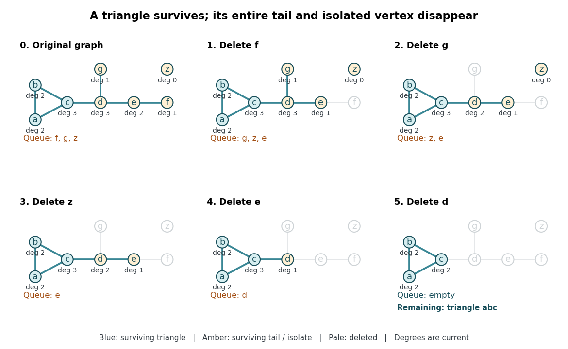
The complete leaf pruning for the 2-core trace: each panel recomputes the displayed degrees of vertices from the surviving induced subgraph, while the FIFO queue determines the next deletion
. Details. A forest has empty 2-core: every nonempty finite forest has an isolated vertex or a leaf of a graph, so deletion cannot stop at a nonempty remainder. In particular, an isolated edge, an isolated vertex, a path graph, and the empty graph all have empty 2-core. Every cycle graph is its own 2-core. Two disjoint triangles in a graph also form their own 2-core, so a 2-core need not be a connected graph; attaching a tree to either triangle changes neither surviving triangle.
Acyclic orientation 2026-10-14
An acyclic orientation is an orientation of a graph whose resulting directed graph has no directed cycle, hence is a Directed acyclic graph. A directed cycle must follow every arrow around its closed route. A cycle in a graph in the skeleton of a directed graph only requires the corresponding undirected edges; their arrows need not agree around the route.
For the same triangle in a graph with vertex set and edges , compareBoth have an undirected cycle in a graph in their skeleton of a directed graph. Only has a directed cycle. In , has no outgoing directed edge, so a route cannot continue from back to .
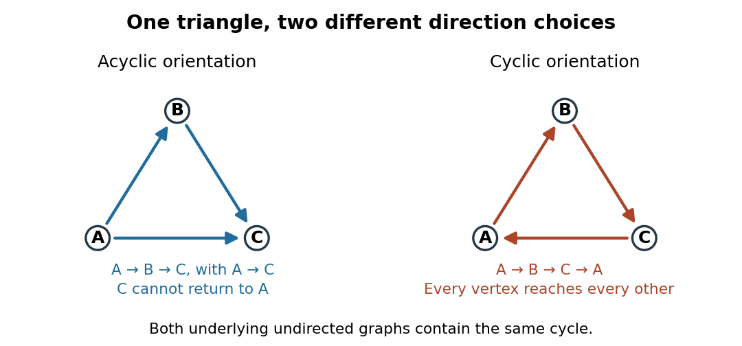
The same triangle in a graph with an acyclic orientation and an orientation of a graph containing a directed cycle
. Details. Thus an acyclic orientation does not require its underlying undirected graph to be a forest. Every orientation of a graph of a forest is acyclic, because a directed cycle would give an undirected cycle in a graph. Conversely, every finite simple graph, including one with many cycles in a graph, admits at least one acyclic orientation by the following ordering construction. On this triangle in a graph, six of the eight orientations of a graph are acyclic; the other two follow the directed cycle in opposite senses.
Adjacency list Created 2026-10-13 Updated 2026-10-20
An adjacency list represents a graph by keeping, for each vertex , a collection of the vertices reached by its outgoing edges. An array indexed by vertex identifiers can locate each collection; the collection itself may use a linked list or an array. In an undirected graph, each nonloop edge supplies an entry at both endpoints.[ref]
Graph.java. Graph.java, class documentation and fields: vertex-indexed adjacency collections; addEdge: entries at both endpoints
For a worked example, take the simple graphwhere denotes the unordered pair . Its adjacency lists, displayed in label order, areThus has three neighbours, although the graph has six vertices. Its list contains exactly the destinations available for a single step from ; no slots are reserved there for . The fourteen neighbour entries represent seven edges, with appearing as in 's list and as in 's list. The label order makes the example easy to read; an adjacency list need not be sorted.
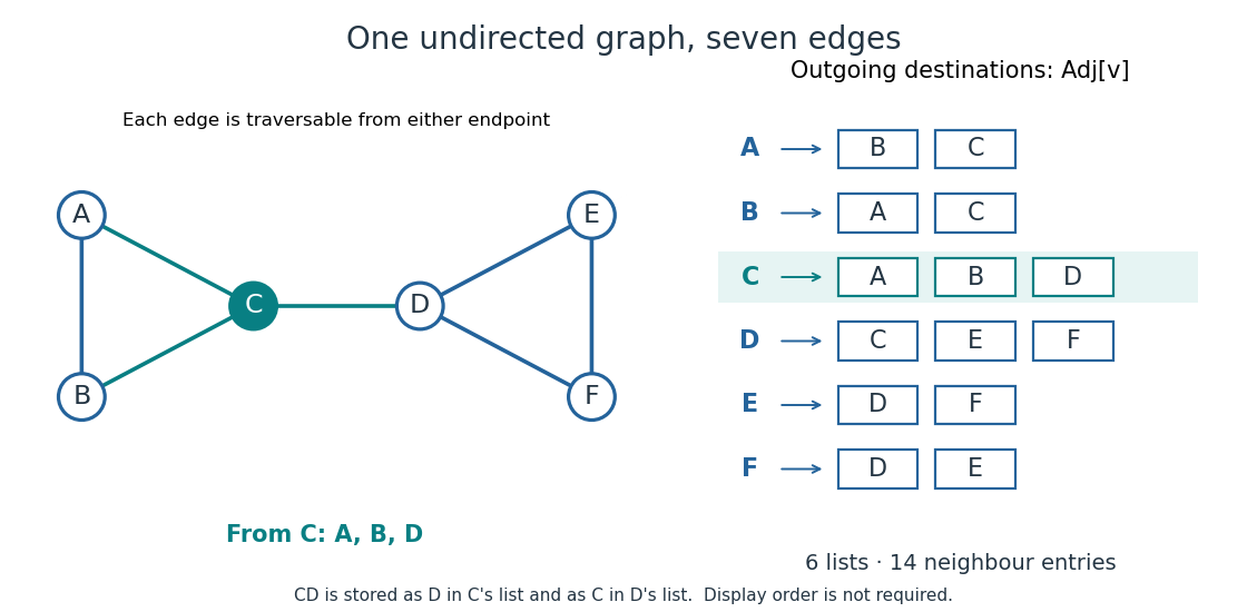
Seven undirected edges and their fourteen adjacency list entries
. Details. The useful idea is to store existing connections explicitly. Neighbour enumeration can then follow exactly the possible next steps, which is what breadth-first search and depth-first search need. In a sparse graph, most pairs of vertices have no edge; adjacency lists avoid reserving a separate adjacency matrix entry for every such absence. Whether this saves work depends on the question: neighbour enumeration and testing one proposed edge have different costs.
Adjacency list edge conventions 2026-10-14
For a directed graph, store in for the edge . The reverse edge is separate and is stored only if it exists. Consequently, list length is outdegree, not indegree, and each directed edge contributes one entry in total. An incoming-list index is additional storage.[ref]
Digraph.java. Digraph.java, addEdge, adj and outdegree: one entry in the tail's collection; indegree is maintained separately
Orient the seven edges of our example from earlier to later labels. The resulting directed graph hasThere are now seven entries, with outdegrees . In particular, needs an empty list even though it is reached from : incoming edges do not make 's outgoing list nonempty. Replacing each directed edge by an undirected graph connection would lose this distinction.
Our running simple graph excludes self-loops and repeated edges. If those restrictions are relaxed, specify how the adjacency list encodes them. Here an undirected self-loop at contributes two copies of to , matching its contribution of two to the degree of a vertex. A directed self-loop contributes one copy, and one each to outdegree and indegree. Distinct parallel edges retain distinct entries; a multigraph's list length can therefore exceed its number of distinct neighbours.[ref]
Graph.java. Graph.java, class documentation: parallel edges and two-entry undirected self-loop convention; addEdge applies both insertions even when v equals w
[ref]Digraph.java. Digraph.java, class documentation and addEdge: parallel edges permitted; a directed self-loop adds one outgoing entry and increments indegree once
For example, add one undirected self-loop at to the seven-edge example. Its list becomes , the vertex degree of becomes four, and the total entry count becomes sixteen for eight edges. If an application instead stores a self-loop once, it must account for its doubled undirected vertex degree separately. In a weighted graph, an entry can be an ordered pair meaning destination and weight ; the weight belongs to the edge, not to the destination vertex.
Bipartite graph Created 2026-09-24 Updated 2026-10-14
A bipartite graph separates its vertices into two independent sets: every edge goes from one part to the other. Here is a finite simple graph and an undirected graph, with no self-loops and no repeated edges. The two parts satisfyThus neither part contains an edge. The parts need not have equal sizes, and some pairs across them may have no edge; requiring every cross pair gives a complete bipartite graph. The independent set and cross-edge definitions are equivalent.[ref]
The Basics (author-hosted chapter preview). Section 1.1, printed p. 3, independent vertices; Section 1.6, printed p. 17, bipartite and complete multipartite graphs
For example, the six-vertex cycle graph with edges has parts and . Drawing the same graph as a hexagon or in two columns changes neither its edges nor its bipartite property. An extra isolated vertex can go in either part.
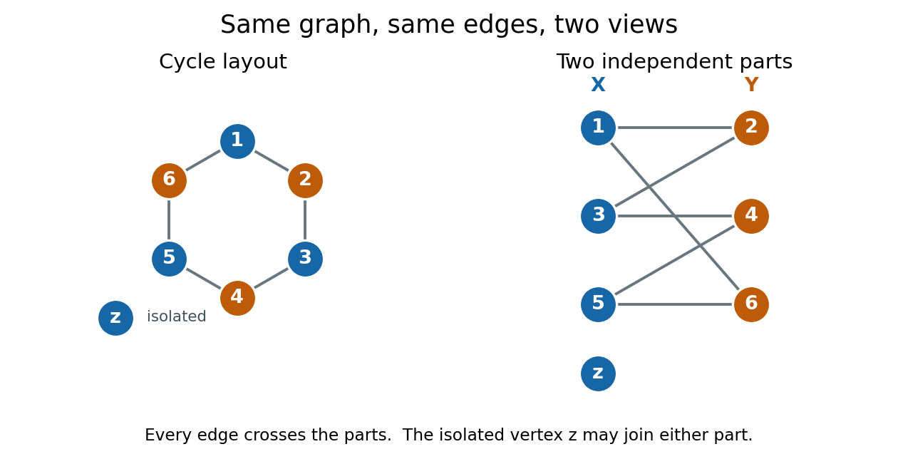
We allow either part to be empty. Consequently a graph with no edges is bipartite, even when ; choose , . Here "two colours" means two colours are available, with no requirement to use both. This convention explicitly includes the empty case, whereas definitions requiring two nonempty classes need an exception. For several connected components of a graph, choose the two parts separately in each graph component and take their unions. In a nonempty connected graph that is bipartite, fixing one vertex's colour forces all others along graph paths, so its two-colour assignment is unique up to swapping the colours. Each graph component, including an isolated vertex, can be swapped independently.
The two-colourability criterion for bipartite graphs identifies these parts with the colour classes of a proper vertex colouring: assign colour to and colour to , so adjacent vertices have different colours. More surprisingly, the odd-cycle characterization of bipartite graphs turns a global requirement into one precise obstruction:This statement is for the finite undirected graph and simple graph model above; a graph cycle has distinct vertices except for the repeated starting vertex. Along a graph cycle in a bipartite graph, colours alternate, so returning to the starting colour takes an even number of edges. Therefore any odd cycle, whether or not other edges join its vertices, prevents a bipartite split.[ref]
The Basics (author-hosted chapter preview). Section 1.6, Proposition 1.6.1 and proof, printed pp. 17–18
Breadth-first search supplies the converse constructively. Start an uncoloured vertex with colour , and use a FIFO queue to explore its graph component. When an edge first discovers , give the opposite colour to , record as its parent in a rooted tree, and enqueue . If both endpoints of any scanned edge already have the same colour, stop with a conflict. Restart from an uncoloured vertex until every graph component has been examined. If no conflict occurs, all edges cross the two colour classes, which are the required independent sets.[ref]
A conflict also explains the failure. In the rooted tree produced by breadth-first search, let be the graph distance from . The colour of is its distance's integer parity. An edge in an undirected graph satisfies , so equal colours force . Follow the two parent chains upward to their lowest common ancestor , discard the shared graph path from to , and join the remaining two graph paths with the conflict edge . The result is a genuine graph cycle withedges, an odd integer. The two branches have no shared vertices except , so this is more than a closed walk. This odd cycle is a certificate that anyone can check directly, using only its listed vertices and edges.
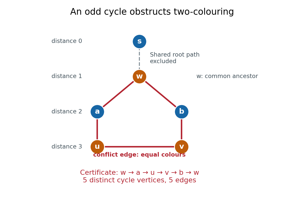
In the example, breadth-first search from gives , , and . The conflict edge closes the odd cycle , with five edges. The common edge is excluded. Thus the same procedure returns either two independent sets covering , or an explicit odd cycle. With adjacency lists and constant-time FIFO queue operations, its time complexity is in Big O notation, with additional storage.[ref]
The two parts often have a practical meaning: workers and jobs, with an edge exactly when a worker can perform a job. A matching in a graph chooses compatible worker–job pairs with no reused endpoint; merely being bipartite does not guarantee enough compatible pairs. Hall's marriage theorem characterizes when every worker can be matched, and the assignment problem adds costs to seek an optimal assignment. These connections make the bipartite structure useful after recognition, as the starting point for selecting edges under constraints.
Breadth-first search Created 2026-09-24 Updated 2026-10-14
Breadth-first search is a graph search that explores successive layers of graph distance from a starting vertex . Here the graph is an undirected graph on a finite set of vertices, and distance counts edges, with no differing edge weights. Mark as discovered, assign , and place it in a FIFO queue. Repeatedly remove the front vertex and scan its adjacency list. Whenever a graph neighbour is still undiscovered, mark it immediately, record as its parent in a rooted tree in the discovery tree, assign , and enqueue at the rear. Marking on insertion ensures that another edge cannot enqueue the same vertex again. [ref]
https://raw.githubusercontent.com/kevin-wayne/algs4/master/src/main/java/edu/princeton/cs/algs4/BreadthFirstPaths.java. Sedgewick and Wayne, Algorithms: BreadthFirstPaths queue and discovery rule
Use the same undirected graph as depth-first search, with vertex set and edgeswhere denotes the unordered pair . Start at and scan graph neighbours in lexicographic order of their one-letter labels. The diagram's generator computes the following layers and the parent in a rooted tree assigned to each discovered vertex; the source is the root of a tree and has no parent in a rooted tree.
| Graph distance from | Vertices in discovery order | Parent in a rooted tree in the same order |
|---|---|---|
| none | ||
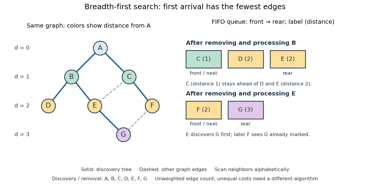
The discovery and removal orders both happen to be . After processing , the FIFO queue is : must be processed before the newer . Processing then skips the already discovered and enqueues , giving . Processing adds nothing. Processing discovers , giving ; later sees already marked and leaves its parent in a rooted tree unchanged. The discovery edges are , forming a rooted tree on all seven vertices even though the original graph contains graph cycles. The discovery tree contains six edges; it need not contain every examined edge.
First arrival is shortest because the FIFO queue keeps assigned distances in nondecreasing order, with entries from at most two consecutive layers. While processing distance , newly discovered vertices receive distance and join the rear. If an undiscovered vertex had a shorter graph path, its preceding vertex on that graph path would lie in an earlier layer and would already have discovered it. Thus is the minimum number of edges from to . This is a mathematical induction over the layers, not an assumption about the drawing. Following the parent in a rooted tree backwards at each step gives ; reverse that sequence to obtain the three-edge graph path . is another shortest graph path, but the specified graph neighbour order makes discover first. Changing that order can change the parent in a rooted tree without changing graph distances. [ref]
https://ocw.mit.edu/courses/6-006-introduction-to-algorithms-fall-2011/1208e162775f6f5cedfbb9f2b694ede0_MIT6_006F11_lec13.pdf. MIT 6.006, lecture 13: distance layers and shortest paths, pp. 4–6
The shortest-route guarantee concerns the shortest path problem measured by edge count. It also minimizes total cost when every edge has the same positive cost. With unequal edge weights, first discovery need not minimize total cost; nonnegative costs can instead be handled by the Dijkstra algorithm. Breadth-first search is useful for minimum-hop routes and for finding all vertices within a specified graph distance. Its FIFO queue finishes an older layer before the next one, whereas depth-first search uses a call stack or explicit LIFO stack to pursue one branch immediately.
With adjacency lists and constant-cost discovery checks, together with constant worst-case or amortized analysis cost for FIFO queue insertion and removal, the time complexity is in Big O notation. Every reached vertex is enqueued and removed once, each incident edge is scanned at most twice in an undirected graph, and initializing all marks and distances takes . The FIFO queue contains at most vertices; the example's maximum is three. Discovery marks, distances and the recorded parent in a rooted tree for each nonroot vertex also give auxiliary space complexity, excluding the graph. An array that shifts every entry on front removal can lose the linear time complexity; the FIFO queue abstraction alone does not make removal constant-cost. Ordering the adjacency lists is a separate preprocessing cost.
A single start reaches only its connected component of a graph. Unreached vertices retain distance and have no recorded parent in a rooted tree. Restarting at each still-undiscovered vertex, while preserving all discovery marks, produces a forest covering the graph; each new root of a tree gets distance zero, so these distances refer to that root of a tree, not to the original .
Chromatic index 2026-10-14
The chromatic index , also called the edge chromatic number, is the least number of labels in a proper edge colouring of a finite undirected graph without self-loops. Equivalently, it is the smallest number of matchings in a graph whose set partition covers all the edges. We take when there are no edges. For an arbitrary edge colouring, one colour always suffices whenever an edge exists, so properness is essential to this definition. The chromatic number instead colours vertices.[ref]
Graph Theory by Reinhard Diestel. Colouring, author-hosted chapter preview, p. 124: chromatic index and line graph
To establish an exact chromatic index, supply both a proper edge colouring and a reason that fewer colours cannot work. Every edge at a fixed vertex must have its own colour, giving the lower bound , where is the maximum degree of a graph. The bound need not be attained: it counts a single resource's workload, while conflicts can also accumulate around a graph cycle.
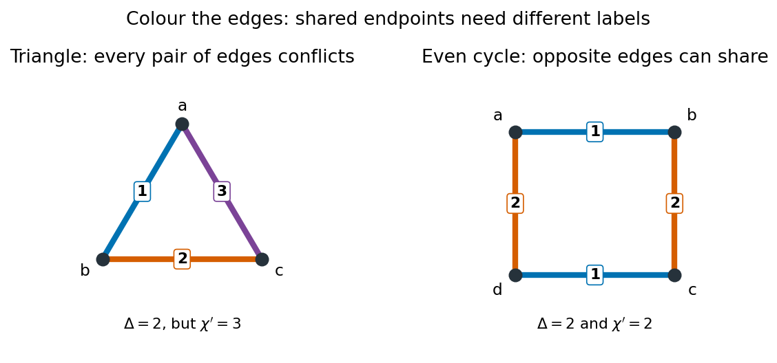
Worked proper edge colourings: a triangle in a graph needs three colours, while an even cycle graph needs two
. Numbers beside edges are colour labels; letters at dots are vertices. Both graphs have maximum degree of a graph two. The triangle in a graph has three pairwise conflicting edges, while opposite edges of the square can share a colour. Details.For the triangle in a graph with edges , every pair of edges shares a vertex, so all three require different labels. The assignment works, proving although . In its line graph, those three edges become a three-vertex clique. Treating this as three pair-resource jobs makes the obstruction tangible: each resource has only two jobs, but every pair of jobs conflicts, so no slot can contain two jobs.
For the square cycle graph with edges , use and . Each colour class is a matching in a graph, and each vertex has one edge of each colour. Since , this proves . More generally, alternation closes on any even cycle graph , . On an odd cycle , , two-colour alternation would make the last and first edges share a colour at their common vertex; a third colour on the last edge suffices. Thus even cycle graphs have chromatic index two and odd cycle graphs have chromatic index three. These exact examples show why maximum degree of a graph alone does not determine the answer.
Closed walk Created 2026-10-06 Updated 2026-10-14
A closed walk is a walk with equal endpoint vertices, . Under our convention this includes the zero-length walk ; returning after traversing at least one edge requires . Closure imposes no other restriction on repeated vertices or edges. In a directed graph, a closed directed walk must also follow every directed edge in its permitted direction.[ref]
Mathematics for Computer Science by Eric Lehman and others. Lehman, Leighton and Meyer, Mathematics for Computer Science, §§9.2 and 11.8.1: closed walks
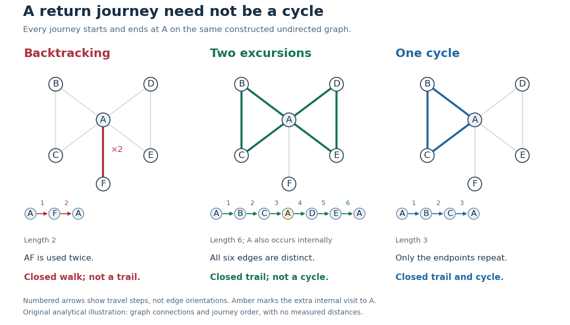
Returning to : backtracking closed walk, closed trail with a repeated internal vertex, and graph cycle
. Details. In the shared simple graph, is a length-two closed walk that immediately backtracks along . It is not a trail, since is used twice, and it is not a graph cycle. The length-six closed walk is a trail, since its six edges are distinct, but is not a graph cycle: it returns to midway through the journey. The length-three closed walk is a graph cycle, with all vertices distinct apart from the required endpoint repetition. In a simple graph that is an undirected graph, a graph cycle has length at least three; the two-step backtrack is excluded.[ref]
Mathematics for Computer Science by Eric Lehman and others. Lehman, Leighton and Meyer, Mathematics for Computer Science, §11.8.1: cycles and backtracking
A positive-length closed walk therefore need not reveal a graph cycle: even a tree permits an out-and-back journey on an edge. A positive-length closed trail in a simple graph does contain a graph cycle. For a proof outline, choose a shortest positive-length consecutive portion of the trail whose endpoint vertices coincide. It cannot repeat an internal vertex, since that would give a shorter such portion; it cannot have length one or two because self-loops and repeated edges are excluded. It is consequently a graph cycle. Cutting it out leaves another closed trail, possibly of length zero, so repetition partitions the original edges into graph cycles. In our six-step example these are the two triangles in a graph. A closed trail using every edge would be an Euler circuit; here is omitted.
Counting return journeys makes closed walks useful even when they repeat edges. For a finite simple graph with adjacency matrix , the walk count from powers of an adjacency matrix gives length- walks from to , for every nonnegative integer . A proof outline is that matrix multiplication appends one allowed step, summing over the previous endpoint; is the identity matrix, recording the unique zero-length walk at each vertex. ConsequentlyThe trace counts closed walks with a specified starting vertex and traversal order, not distinct graph cycles. These formulas use adjacency entries, not arbitrary travel costs in a weighted graph.[ref]
https://ocw.mit.edu/courses/14-15-networks-spring-2022/mit14_15s22_lec2.pdf. Alexander Wolitzky, Graph Theory and Social Networks, slides 9–10: powers of adjacency matrices
In our example, : the five length-two closed walks are , , , , and . Also , going round either triangle in a graph in either direction, and : each of the two triangles in a graph supplies three choices of starting vertex and two directions. These exact counts for the constructed graph illustrate why return counts and graph cycle counts differ.
A closed walk naturally models a delivery or inspection journey that returns to its depot. Repeated vertices let it combine several excursions; repeated edges let it serve a dead end and return. For an Euclidean travelling salesman tour, one can first construct a closed walk visiting all locations and then use the triangle inequality to shortcut repeated visits without increasing total length. That argument assumes direct travel between the retained locations is permitted, as in a complete graph weighted by Euclidean distance; an arbitrary road network need not contain those shortcut edges.
Constraint graph 2026-10-25
For a binary constraint satisfaction problem, the undirected graph with one vertex per variable and an edge for each variable pair sharing a binary constraint. Unary conditions restrict constraint domains but add no edges. A more general constraint can be represented in a primal constraint graph by joining every pair of variables in its scope; such edges do not make a genuinely many-variable constraint binary.
After restricting constraint domains, a binary constraint can become automatically satisfied for every remaining pair of values. Removing such constraints can reveal a tree and enable tree-structured constraint satisfaction.
Cut vertex Created 2026-10-06 Updated 2026-10-14
A cut vertex, also called an articulation point, is a vertex of an undirected graph whose deletion increases the number of connected components of a graph. Write for that count, including isolated vertices, and for the graph obtained by removing and every incident edge. Then the test is , even when the original graph is disconnected. By contrast, deleting a bridge in a graph removes just one edge and keeps both endpoint vertices. These are different failure models. [ref]
https://algs4.cs.princeton.edu/41graph/. Sedgewick and Wayne, Algorithms, §4.1: bridges and articulation points
First take two triangles in a graph, and , sharing only the vertex . This simple graph hasHere abbreviates the unordered pair . Removing leaves the two connected components of a graph and , so . Removing any other vertex leaves a connected graph. Thus is the only cut vertex. Every edge lies on a triangle in a graph, so deleting any single edge still leaves a graph path between its endpoints along the other two edges. There are no bridges in a graph.
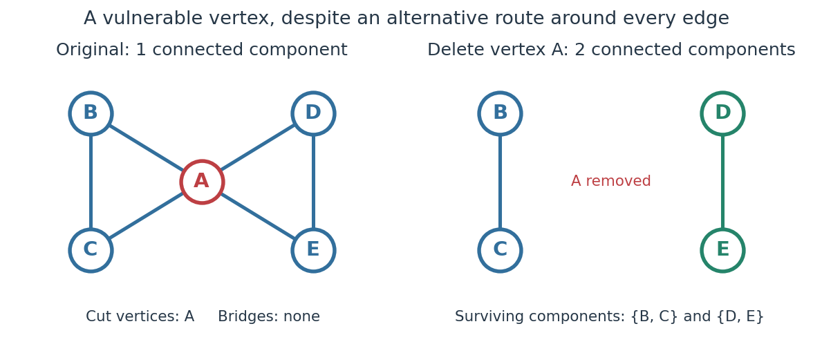
The generator computes the adjacency lists and checks every vertex deletion, giving the following complete table:
| Deleted vertex | Original graph neighbours of | |
|---|---|---|
Now take two disjoint triangles in a graph, and , joined by the edge :Deleting only preserves all six vertices and leaves connected components of a graph and : is the only bridge in a graph. Deleting also removes and , leaving connected components of a graph and . Deleting instead leaves and . Thus are exactly the cut vertices.
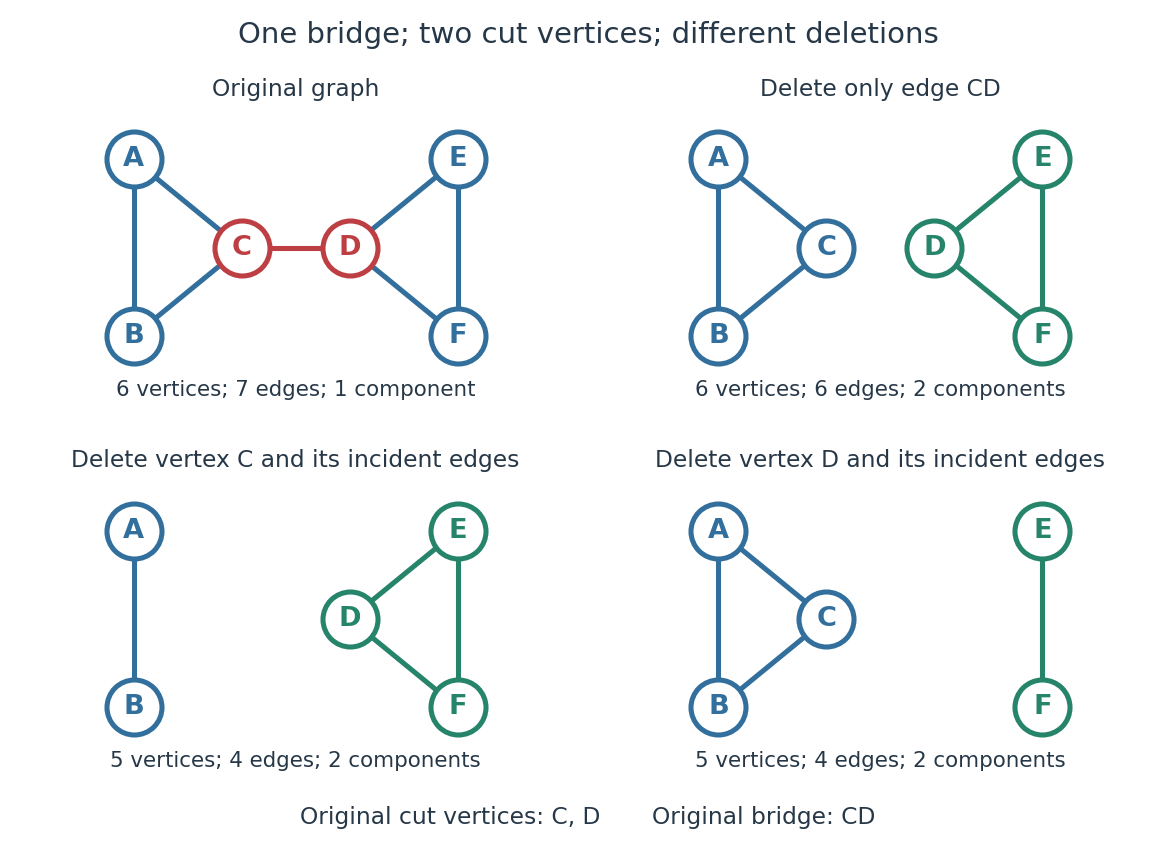


Again the adjacency lists and all vertex deletion counts are computed directly:
| Deleted vertex | Original graph neighbours of | |
|---|---|---|
For a disconnected example, adjoin an isolated vertex to the first graph. Now , deleting gives , and deleting gives . The original graph was already disconnected, but is still a cut vertex; is not. The empty graph has count zero, so deleting the only vertex of a one-vertex graph does not create a cut vertex. Nor is either endpoint of a single isolated edge a cut vertex, although that edge is a bridge in a graph.
In a communications network, a cut vertex models a router whose failure separates surviving routers. The shared- example shows why having an alternative graph path around each individual edge does not protect against failure of the common router. An additional edge from to removes this particular vulnerability: after deleting , still join the two sides. A bridge in a graph instead models a vulnerable link. This distinction tells us whether to add another cable between existing devices or a route avoiding an indispensable device; it describes connectivity, rather than traffic capacity or failure probabilities.
The beautiful structural consequence is that a graph splits into biconnected components joined at cut vertices. Within each nontrivial robust piece, a single vertex failure cannot separate the other vertices; between pieces, the shared cut vertices reveal the bottlenecks. Also, a Hamiltonian graph has no cut vertex: deleting any vertex from its Hamilton cycle leaves a Hamiltonian path through all remaining vertices.
Historically, Tarjan's June 1972 paper developed depth-first search as a tool for finding biconnected components in time linear in the numbers of vertices and edges. [ref]
https://epubs.siam.org/doi/10.1137/0201010. Robert Tarjan, Depth-First Search and Linear Graph Algorithms, SIAM Journal on Computing 1(2), 146–160 (1972)
In his 1983 recollection, Tarjan credited Hopcroft with the original linear-time biconnected component algorithm during their collaboration beginning in summer 1970, and described the published version as a refinement. The historical lesson is how a carefully organized traversal turns many separate deletion experiments into one computation. [ref]https://garfield.library.upenn.edu/classics1983/A1983QY47200001.pdf. Robert E. Tarjan, Citation Classic recollection (1983)
Depth-first search Created 2026-10-13 Updated 2026-10-20
Depth-first search is a graph search that follows a branch as far as it can before returning to try the next unexplored branch. Starting at a vertex of an undirected graph on a finite set of vertices, mark as discovered. Scan its graph neighbours in a fixed order: for each undiscovered vertex, record the current vertex as its parent in a rooted tree in the discovery tree, mark the new vertex, and explore it immediately using recursion. Return when its adjacency list is exhausted. Discovery marks persist after return, preventing a graph cycle from causing repeated exploration. This branch-and-return rule is the maze exploration described in MIT's notes. [ref]
Use the same unweighted undirected graph as breadth-first search, with vertex set and edgeswhere denotes the unordered pair . Visit graph neighbours in lexicographic order of their one-letter labels, starting at . The discovery order, computed by the diagram's generator, isThe discovery edges in order are . They form a rooted tree spanning the reached vertices, with root of a tree . The other edges, and , remain in the original graph but never discover a new vertex. In particular, the graph cycle causes no repeated discovery.
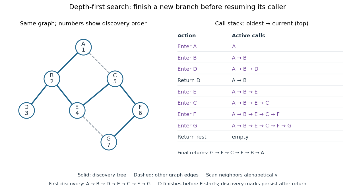

At there is no undiscovered graph neighbour, so its call returns to . The next call enters , then , then , then . Immediately after discovering , the call stack is , with on top; is still discovered but its call has finished. The maximum call stack depth is six, although seven vertices are discovered. Following the recorded parent in a rooted tree backwards at each step reconstructs a graph path; here the route from to is , using five edges. Breadth-first search instead finds , using three edges. Depth-first search establishes reachability but does not guarantee the fewest edges.
An explicit LIFO stack can replace recursion, but its entries and discovery rule must be specified. To reproduce this exact traversal, store one frame per active vertex, retaining the next position in its adjacency list. Advance the top frame by one graph neighbour; if that vertex is undiscovered, mark it and push its frame immediately; pop an exhausted frame. Pushing all undiscovered graph neighbours at once and marking them on push is a different iterative variant. Even pushing them in reverse lexicographic order does not generally reproduce the parent in a rooted tree relationships above: would already be marked while processing , so could not discover .
With an adjacency list representation, constant-cost discovery checks and frame operations, and the graph neighbours already ordered, depth-first search has time complexity in Big O notation. Each reached vertex is entered once and each incident edge is examined at most twice in an undirected graph; initializing all discovery marks costs . The call stack has depth at most , since no active vertex repeats. Discovery marks and the recorded parent in a rooted tree for each nonroot vertex also need auxiliary space complexity, excluding storage for the graph. Sorting adjacency lists to obtain a chosen order is additional work. [ref]
https://raw.githubusercontent.com/kevin-wayne/algs4/master/src/main/java/edu/princeton/cs/algs4/DepthFirstPaths.java. Sedgewick and Wayne, Algorithms: DepthFirstPaths discovery marks and resource bounds
One start explores only its connected component of a graph. To cover a disconnected graph, start again at every still-undiscovered vertex while keeping all discovery marks; the discovery trees form a forest. Depth-first search is useful for reachability, constructing a spanning tree of a connected graph, and organizing the return steps needed by a depth-first traversal of a tree. For detecting a graph cycle in a simple graph that is an undirected graph, an edge to an already discovered vertex other than the current parent in a rooted tree closes a graph cycle; the immediate return edge to that parent in a rooted tree is not itself a graph cycle.
// Target: computer-science.bigb
DFS lowpoint 2026-10-14
For a finite simple graph that is an undirected graph, the DFS lowpoint of is the smallest DFS discovery time reachable by following zero or more discovery edges down its rooted tree, then at most one non-discovery edge to an ancestor. Staying at is allowed. Ignore the reverse traversal of the discovery edge to the parent in a rooted tree: it is the same edge, not an escape route. Start with . On returning from a child in a rooted tree , replace by . For a non-discovery edge from to an earlier ancestor , replace it by . This summarizes how far upward the explored branch can reconnect. [ref]
https://sites.cs.ucsb.edu/~gilbert/cs240a/notes/TarjanDFS.pdf. Tarjan (1972), §3, LOWPT recurrence, pp. 151–153
The cut vertex criterion has a separate case for each root of a tree in the discovery forest:
- A nonroot vertex is a cut vertex exactly when some child in a rooted tree satisfies .
- A root of a tree is a cut vertex exactly when it has at least two children in a rooted tree, counting discovery edges, rather than all graph neighbours.
- A discovery edge is a bridge in a graph exactly when . A non-discovery edge is never a bridge in a graph.
Why does equality matter? If , the branch below can reconnect to , so the discovery edge lies on a graph cycle and is not a bridge in a graph. Deleting the vertex destroys that reconnection too. If has a parent in a rooted tree, the branch is then separated from that parent in a rooted tree, explaining the non-strict cut vertex test. For a root of a tree, there is no earlier side to separate from; distinct discovery branches cannot have an edge between them, since depth-first search would have explored them as one branch. This gives the two-children in a rooted tree rule. These are proof outlines of the criteria. [ref]
https://algs4.cs.princeton.edu/41graph/Biconnected.java.html. Sedgewick and Wayne, Biconnected.java: discovery, lowpoint and root tests
[ref]In the joined- example with DFS discovery times , the DFS lowpoints in label order are . For and its child in a rooted tree , : is a bridge in a graph, and is a cut vertex. For and its child in a rooted tree , : is a cut vertex, although is not a bridge in a graph. The root of a tree has only one child in a rooted tree, , so it is not a cut vertex. In the shared- example, the root of a tree has two children in a rooted tree, and , and is a cut vertex, while every DFS lowpoint is and no edge passes the strict bridge in a graph test.
Restart depth-first search at every undiscovered vertex to cover a disconnected graph, applying the root of a tree rule separately in each connected component of a graph. With adjacency lists and constant-cost label operations, computing all DFS lowpoints, cut vertices and bridges in a graph has time complexity in Big O notation, because each vertex is discovered once and each edge is inspected twice. The simple parent-skipping rule assumes a simple graph. In a multigraph, skip only the actual parent edge, identified individually: a parallel edge to the same parent in a rooted tree is a valid reconnection and can prevent the first edge from being a bridge in a graph. The criteria here concern undirected graphs; a directed graph requires a different connectivity analysis.
Diffusion on a graph 2026-10-14
The continuous-time diffusion model on a finite undirected graph uses the Graph Laplacian in the ordinary differential equationAcross each edge, the higher value sends an amount proportional to the difference to the lower value. The two contributions cancel in the sum over vertices, giving conservation of mass:If the entries represent masses, start with nonnegative entries; signed entries can instead describe deviations from a common level. For the three-vertex path graph, the initial vector is an eigenvector with eigenvalue one, so the exact solution isMore generally, an eigenvector with eigenvalue decays by . The spectral theorem for real symmetric matrices supplies an orthonormal basis of these eigenvectors, and the kernel of a graph Laplacian identifies the surviving terms. On a nonempty connected graph,The limiting value is the original arithmetic mean. On a disconnected graph, each connected component of a graph converges to its own original arithmetic mean. The same matrix therefore measures neighbour disagreement, detects disconnected regions and governs relaxation toward agreement.
Dijkstra algorithm 2026-10-14
The Dijkstra algorithm solves the single-source shortest path problem in a finite graph with nonnegative edge weights, finding distances to all reachable vertices. Start with tentative distance and elsewhere. Repeatedly choose the unfinalized vertex with least tentative distance, declare that label permanent, and perform edge relaxation on its outgoing edges. For an undirected graph, inspect both directions. A finite tentative distance always records the cost of a discovered graph path, but can improve before finalization.
In our example, finalizing discovers at , at , and at . Choose next: edge relaxation through lowers to and to . Choose : edge relaxation through lowers to . Finally choose . The permanent distances are therefore , , , ; the evolving tentative distances were and .
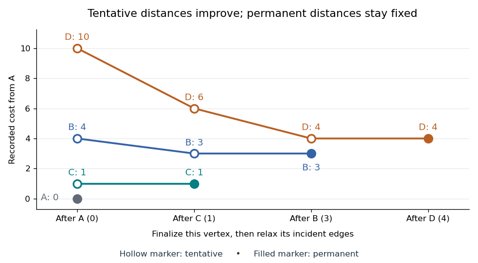
Tentative distances fall until the Dijkstra algorithm makes each label permanent
. Details. 
Store a shortest-path predecessor whenever edge relaxation improves a label. The final table contains enough information to reconstruct routes, rather than merely their costs:
| Vertex | Distance from | Shortest-path predecessor | Finalization order |
|---|---|---|---|
| None: source | |||
Following shortest-path predecessors backwards gives ; reversing the order gives . If only this destination matters, stop when is finalized. Stopping when is first discovered would incorrectly return . If the smallest remaining tentative distance is , all remaining vertices are unreachable.
Why is the permanent choice safe? Suppose the selected vertex had a cheaper graph path. Let be the first unfinalized vertex on that graph path. Its preceding vertex was finalized, so edge relaxation has already offered a label no larger than that prefix's cost. Nonnegative remaining edge weights make the whole cost at least this prefix's cost; selection gives . A cheaper graph path would contradict these comparisons. Zero weights are allowed; ties can be resolved arbitrarily. This is the reason the label-setting shortest-path algorithm works, rather than a lucky feature of the drawing.
Negative weights break that reasoning. In a directed graph with costing , costing , and costing , the Dijkstra algorithm would finalize at before discovering the cheaper cost . The Bellman-Ford algorithm handles negative edge weights when no relevant negative directed cycle exists.
With an adjacency list and an indexed binary heap implementing a priority queue, the time complexity is for , using Big O notation. Each vertex is extracted at most once, each edge is inspected once per direction, and each successful edge relaxation decreases a heap key in time. This assumes constant-cost arithmetic and comparisons; exact computation with very large weights adds their representation cost. The queue uses space beyond the graph. Simply scanning all remaining vertices gives instead.[ref]
https://algs4.cs.princeton.edu/44sp/DijkstraSP.java.html. Princeton, DijkstraSP implementation
[ref]https://algs4.cs.princeton.edu/code/javadoc/edu/princeton/cs/algs4/IndexMinPQ.html. Princeton, indexed binary heap operations
The 1959 paper presents the shortest path problem as its second problem, after the minimum spanning tree problem, and grows known shortest routes in increasing distance order.[ref]
https://www.cs.yale.edu/homes/lans/readings/routing/dijkstra-routing-1959.pdf. Dijkstra, A note on two problems in connexion with graphs, pp. 269–271
In his later recollection, Dijkstra dated the shortest-route discovery to 1956: a demonstration for the ARMAC computer used a simplified Dutch railway map and printed the route between towns. A practical request became an enduring algorithm because the same distance rule applies to any suitable graph.[ref]https://garfield.library.upenn.edu/classics1983/A1983QA19900001.pdf. Dijkstra's recollection, published in 1983
Eulerian graph Created 2026-09-24 Updated 2026-10-14
An Eulerian graph has an Euler circuit: a closed trail traversing every edge exactly once. Here the graph is a finite undirected graph, possibly a multigraph with self-loops. Parallel edges retain distinct identities, and each self-loop contributes two to its vertex degree. Repeated vertices are allowed. This models inspecting every road segment once, even when a junction must be revisited.
For a nonempty set of edges, the Euler circuit criterion requires a connected graph only on the edge support of a graph: isolated vertices impose no travel requirement. A single vertex with a self-loop and two vertices joined by two parallel edges are both Eulerian graphs. Neither requires three vertices. With no edges and at least one vertex, we allow the zero-length trail at that vertex as an Euler circuit; the graph with no vertices has no such walk.
The motivating Seven Bridges of Königsberg problem asks for an Eulerian trail, which need not return to its starting vertex. In Leonhard Euler's Solutio problematis ad geometriam situs pertinentis by Leonhard Euler, §2 poses the bridge-crossing question and §§4–6 encode land regions by letters. The river's shape drops out: only the connections matter. The paper was written in 1735 and published in 1741, according to the Euler Archive; the journal volume carries the nominal year 1736.[ref]
Forest Created 2026-09-24 Updated 2026-10-14
A forest is an undirected graph with no graph cycle; each of its connected components of a graph is a tree, including any isolated vertex. A finite forest with vertices and connected components of a graph hasIndeed, a connected component of a graph with vertices contributes edges; adding these counts gives . Equivalently, start with isolated vertices: every added edge must join different connected components of a graph, reducing their number by one. Joining vertices already connected would create a graph cycle. [ref]
https://ocw.mit.edu/courses/18-200-principles-of-discrete-applied-mathematics-spring-2024/mit18_200_s24_lec05-06.pdf. MIT, counting notes, p. 4: building forests by merging components
Deleting in our example gives , , and five edges: the two trees contribute . Deleting as well leaves isolated, so and four edges. A forest therefore describes separate hierarchies or the intermediate stages of building a spanning tree. The acyclic graph condition accounts for missing connections without assuming that all locations are mutually reachable.
Graph coloring Created 2026-10-14 Updated 2026-10-20
A graph coloring assigns labels called colours to elements of a graph, subject to specified constraints. Here we focus on proper vertex colouring of a simple graph : it is an undirected graph with a finite set of vertices, and a colouring with at most colours is a functionThe colour labels need not be visual colours: they can represent time slots or resources. Unused labels are allowed. Properness concerns graph adjacency, so moving vertices in a drawing does not change whether the graph coloring is valid.[ref]
https://ocw.mit.edu/courses/6-1200j-mathematics-for-computer-science-spring-2024/mit6_1200j_s24_lec11.pdf. MIT, Graphs and Coloring, Section 2.1
Each colour class is an independent set: no edge has both endpoints in it. Conversely, a set partition of into independent sets gives a proper graph coloring by assigning one colour to each part. Thus graph coloring groups mutually compatible objects, and its chromatic number asks for the fewest such groups.
For an illustrative scheduling model, let each vertex represent an activity of equal duration and each edge represent a pair that cannot occur in the same time slot. A proper graph coloring is then a schedule respecting those pairwise conflicts. If the conflicts form a cycle graph with edges , activities can share one slot and another. This model assumes interchangeable slots and includes only the pairwise conflicts encoded by the graph.[ref]
https://ocw.mit.edu/courses/6-042j-mathematics-for-computer-science-fall-2010/1ccaf180bcd244fddd32e60789fa922f_h9wxtqoa1jY.pdf. Leighton, MIT Graph Theory and Coloring, transcript pages 8–10
The word "colouring" also occurs in edge coloring, which requires different colours on edges sharing an endpoint. The chromatic number discussed here always refers to proper vertex colouring.
Graphic matroid 2026-10-14
For a finite undirected graph, the graphic matroid has its edges as the ground set. A subset is a matroid independent set when its edges form a forest on the original vertices, including isolated vertices. Its matroid bases give a spanning tree in each connected component of a graph; for a connected graph, each matroid basis is a spanning tree.
For a graph triangle on vertices , label the edges , , and , with weights . The empty set, all singletons, and all pairs are forests; the triple contains the graph cycle . Thus its eight subsets have exactly the independence pattern checked in the weighted three-vector matroid, and the same fifteen exchange comparisons pass. The matroid greedy algorithm chooses , chooses , and rejects , producing the heaviest spanning tree, of weight .
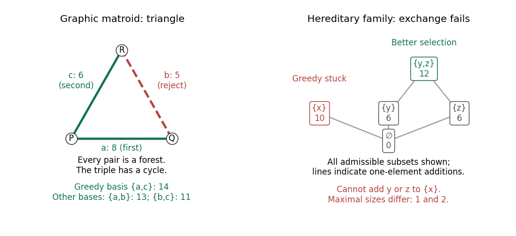
A weighted graph triangle admits greedy selection of a matroid basis; a hereditary independence system without exchange traps a greedy algorithm at weight instead of
. Details. 
Exchange outline. Deleting edges cannot create a graph cycle. If forests have , some edge of joins different connected components of a graph of : otherwise, within each such component, would have at most its number of vertices minus one edges, giving . Adding that edge keeps a forest. This is the matroid independence axioms expressed through connectivity.
Induced subgraph game 2026-10-25
A transferable utility game represented by a weighted undirected graph, with one player per graph vertex. A coalition receives the sum of weights of the graph edges in its induced subgraph; absent edges have weight zero. Singleton and empty coalitions have value zero. This is a representation of a transferable utility game, distinct from a graphical description of local payoffs in a normal-form game.
Laplacian matrix Created 2026-10-14 Updated 2026-10-20
The Graph Laplacian converts local differences along edges into a linear map. Throughout this section, is a finite undirected graph with no self-loops or repeated edges, and each edge has weight one. In a fixed order of vertices, let be the adjacency matrix and the degree matrix. The combinatorial Graph Laplacian isThus the value at a vertex is compared with its neighbours. Every row sums to zero, so : a constant vector produces no differences. This definition and the associated Graph Laplacian quadratic form are developed in Spielman's authored survey.[ref]
https://www.cs.yale.edu/homes/spielman/PAPERS/SGTChapter.pdf. Spielman, Spectral Graph Theory, Sections 16.3.1–16.3.2
For the three-vertex path graph , the vertex degrees are , and in that orderDirect multiplication gives three eigenvectors and their eigenvalues:The constant eigenvector has eigenvalue zero; the other two describe progressively stronger neighbour disagreement. Dividing these eigenvectors by , respectively, gives an orthonormal basis. The four-vertex cycle graph is already worked out under circulant matrix, where Fourier diagonalization of a circulant matrix gives its eigenvalues.