Choose a basis of the two-dimensional abelian Lie algebra , and lifts with the same names. Every alternating bilinear form is determined by , and every such form is a Lie algebra two-cocycle because every Lie bracket in is zero. Thus every central extension of a Lie algebra has a basis with
If , all Lie brackets vanish, so this is the direct sum of Lie algebras . If , replace the central basis vector by . Then , which is the Heisenberg Lie algebra . This change of basis shows that every nonzero gives the same Lie algebra isomorphism class.
These two Lie algebras cannot be isomorphic: their derived algebras have dimensions zero and one, respectively, and a Lie algebra isomorphism preserves the derived algebra. Moreover, the Heisenberg Lie algebra cannot be a direct sum of Lie algebras , since that direct sum of Lie algebras would have zero Lie bracket. Therefore
Here “up to isomorphism” means the Lie algebra isomorphism class of the middle Lie algebra, allowing a change of the identifications at the ends of the short exact sequence. If instead equivalence of central extensions of a Lie algebra must induce the identity on both and , the parameter cannot change: the formula in part (a) has . That stricter notion has one class for each , rather than two. This distinction explains the convention required by the question.
Since the general linear Lie algebra has zero Lie bracket, identify it with . A central extension of a Lie algebra is a short exact sequence
of Lie algebra homomorphisms with contained in the center of a Lie algebra . Thus is surjective, its kernel is precisely the indicated line, and that line commutes with all of .
Choose a linear map with . Such a section exists by lifting a basis. Identify with the direct sum of vector spaces by . The difference belongs to the kernel of , so there is a unique bilinear map such that
It is an alternating bilinear form: , equivalently in characteristic zero. Taking the central component of the Jacobi identity gives the Lie algebra two-cocycle condition
Conversely, any alternating bilinear form satisfying this identity defines a Lie algebra by
Indeed its Lie bracket is an alternating multilinear map and a bilinear map, and the two components of its Jacobi identity are respectively the Jacobi identity in and the displayed Lie algebra two-cocycle condition. The line is central, and projection to gives the required central extension of a Lie algebra.
For later use, replacing by , where is in the dual space, changes the Lie algebra two-cocycle to
Thus changes of section add a Lie algebra two-coboundary, up to the conventional sign. A section that is a Lie algebra homomorphism has and gives a direct sum of Lie algebras.
Encode by phase zero and by phase . Alice and Bob choose their bits independently and keep their choices private. Bob announces the trial numbers with a D0 click over an authenticated public channel. For each retained trial, c guarantees that their bits agree. In the ideal symmetric setup, the two equal-phase cases and give the same click probability, so announcing success does not itself reveal which shared bit was used.
The matching-phase cases occur with probability , and a matching case succeeds with probability . Therefore
For independent ideal trials, the raw-key length has a binomial distribution with standard deviation . These are bits before sacrificing test positions or performing privacy amplification.
A missing click does not certify unequal phases: the same phases also fail to click with probability . With uniform choices,
Thus a no-click trial supplies neither a known equal bit nor a known complemented bit. This is why it cannot be retained by the direct error-free sifting rule. The source's “cannot use” should be understood in this sense: the events are not statistically independent, so an absolute claim that they contain no information would be false.
To obtain a secret final key, reveal and discard a random subset of retained bits to test the observed error rate, then apply reconciliation and privacy amplification as required by a security analysis of the actual implementation. Resolving which time path a photon took removes the accepted histories' quantum coherence and can turn destructive interference into false D0 clicks, providing a simple disturbance test. Equal-phase click correlations alone are not a proof of security against every attack, particularly in the presence of losses and device imperfections. The supplied ideal model fixes the sifted rate ; it does not fix a positive secure final length without an adversary model and observed parameters.
Let denote immediate transmission through the BS1 subsystem between Bob's lower-right port and Alice's upper-left port; let denote transmission after one visit to each internal mirror. From the same beam splitter rules as in b, the corresponding amplitudes in either direction are
up to a common fixed two-mirror propagation phase. The minus sign in comes from the or reverse scattering. The two paths selected by D0's time gate are on the outward journey followed by on the return, and outward followed by on the return. They have the same total delay and fixed propagation phase, so their probability amplitudes interfere.
For the first history, Alice applies to the late component, while Bob's return-time modulation is not encountered in the return delay arm. For the second, Alice's early component is unmodulated and Bob applies in the return delay arm. Bob must time his modulation to the return passage, leaving the outward reference preparation unchanged; this is implicit in the stated encoding. Each enabled modulator is traversed twice, so its single-pass phase becomes the stipulated .
Include the amplitude to enter BS1 through BS2, and the amplitude of modulus to reach D0 through BS2 on return. Both histories therefore contain six 50:50 beam splitter factors. Ignoring one common unobservable global phase,
Hence the unconditional probability per emitted photon, with no renormalization after discarding paths, is
For the allowed values , this is when and zero otherwise. The ignored trajectories exit other ports or other time bins; excluding them from D0's acceptance does not increase the success probability. Equal mirror reflection phases, channel phases and Alice's mirror phase multiply both accepted histories equally and cancel from the interference condition. A residual relative phase would need calibration.
Starting at port 1, the first beam splitter encounter sends amplitude straight out through port 0 and stores amplitude towards M2. A return from M2 enters port ; it sends the stored amplitude times out through port 1 and times towards M1. A return from M1 enters port ; it sends amplitude times out through port 0 and times towards M2. Both internal continuations carry , so two additional encounters multiply the surviving amplitude by .
With the fixed mirror and propagation phases absorbed as in a, the nonzero coefficients of the outgoing single-photon state are
and . The first nonzero terms are , , and . If fixed reflection amplitudes are retained instead, multiply by and by , as well as the appropriate delay propagation phases. These unit-modulus factors do not alter the following probabilities.
Distinct exit events are orthogonal because they differ in output port or arrival-time bin. This requires the incident wavepacket to resolve the delay. Summing the squared moduli as geometric series gives
Their sum is one. After encounters the probability of still being inside is , which tends to zero, so no trapped component is omitted.
The source drawing places the delay line in the M2 arm. A visit to M2 crosses that line in both directions. If is its one-way delay, then an exit after encounters has crossed it times:
If the phrase “delay time ” instead denotes the complete M2-arm round-trip delay, replace by in the floor formula. The wording does not explicitly distinguish these conventions. Consecutive encounters can produce the same exit time in different ports: for example both follow one M2 visit. If the incident wavepacket were much longer than the arm delay, different histories in the same port would overlap and their probability amplitudes would have to be added before squaring; the asserted time-bin expansion would then not be an orthonormal event basis.
The two output ports are orthogonal single-photon states. Conservation of total probability at a lossless beam splitter gives . With real and positive,
In the ordered input basis and output basis , the beam splitter scattering matrix is
For the usual reciprocal lossless beam splitter, reversing propagation uses . Consequently,
The relative phase in the first rule is essential to the repeated-path calculation. Overall port phases may be changed consistently; they cannot be changed on one pass alone while retaining the original scattering rules. In the following, take unit mirror reflection amplitudes by incorporating fixed reflection phases into the propagation-mode convention, and keep any unremoved propagation phase explicitly if needed.
Yes. Replace the target qubit by a register of qubits and implement the controlled unitary gate
The algebra in c uses only normalization and unitarity, so for an arbitrary pure register quantum state it still gives . For a mixed register quantum state , linearity gives . With ,
Only the control qubit needs to be pure. A uniformly randomized computational basis preparation supplies the target maximally mixed state. This is the principle of trace estimation by a maximally mixed Hadamard test. The extension is algebraic; efficiently implementing controlled- still requires a known suitable gate construction. Moreover, estimating the unnormalized trace to fixed additive precision requires increasingly precise estimation of the normalized signal as grows. There is no automatic efficient reconstruction of all entries of .
For second-qubit inputs and , c gives control expectation values and . Preparing the maximally mixed state is equivalent to choosing these inputs independently with equal probability and discarding the choice. Linearity of the density operator evolution and quantum measurement probabilities therefore gives
Hence
The factor two is essential: the Hadamard test directly estimates the normalized trace. More generally, a target density operator gives . This argument never requires knowledge of the eigenvectors of .
Read the source network as a Hadamard test: a Hadamard gate on the first qubit, a controlled unitary gate with the first qubit as control, and another Hadamard gate on that control. Starting from , the successive quantum states are
Apply b to the last line. Since by unitarity,
For the Pauli Z gate observable on the first qubit, the two eigenvalues are and . Thus
As a check, returns outcome zero certainly, while returns one certainly. The controlled unitary gate makes this relative phase measurable even though multiplying an isolated system's quantum state by is only a global phase.
Expand the possibly unnormalized second-qubit kets as and . The joint quantum state is
The Born rule in the orthonormal computational basis gives , , and similarly for the two outcomes beginning with one. Ignoring the second outcome therefore gives
Equivalently these are the squared norms of and . Orthogonality of the first qubit's basis gives , even if is nonzero. For a nonzero-probability outcome, the conditional second-qubit quantum state is the corresponding ket divided by .
Assume . Let Alice's first recorded quantum measurement outcome be . Immediately afterward she assigns the conditional pure quantum state , with probabilities , . Bob, who has no record, assigns the density operator
This is a nonselective quantum measurement, which removes the initial computational basis coherence. It is not generally the original pure quantum state.
After the Hadamard gate, Alice assigns for , or for . Bob assigns
Both and give either final computational basis outcome with probability . Thus, after Alice records the second outcome , she assigns , whereas Bob assigns
Alice's conditional quantum states are pure; Bob's are averages over her unobserved records. They agree on all probabilities when supplied the same information. Their first descriptions can coincide if the initial quantum state is a computational basis state; after the second quantum measurement, Bob's maximally mixed state differs from each conditional pure quantum state.
In liquid-state NMR quantum computing, use two distinguishable spin- atomic nuclei in one molecule as the two qubits. Their different resonance frequencies permit selective radiofrequency pulses for one-qubit rotations. In a suitable rotating frame, refocusing removes unwanted one-spin terms while the NMR scalar coupling supplies
Assuming , free evolution for implements . Define . Then
This equality follows directly by evaluating the four diagonal entries: the first three are and the entry is . Negative can be handled by refocusing or reversing the effective interaction sign. The global phase can be ignored.
Thus the marked-state phase oracle for requires scalar-coupling evolution and calibrated one-spin rotations. For a marked word , conjugate by , realized as selective pulses. The Grover diffusion operator uses the same entangling operation with additional one-qubit pulses. Liquid-state NMR quantum computing usually reads an ensemble signal and often prepares an effective pseudo-pure deviation from a large mixed background; that reproduces this small quantum algorithm's signal without providing a scalable source of pure initialized qubits.
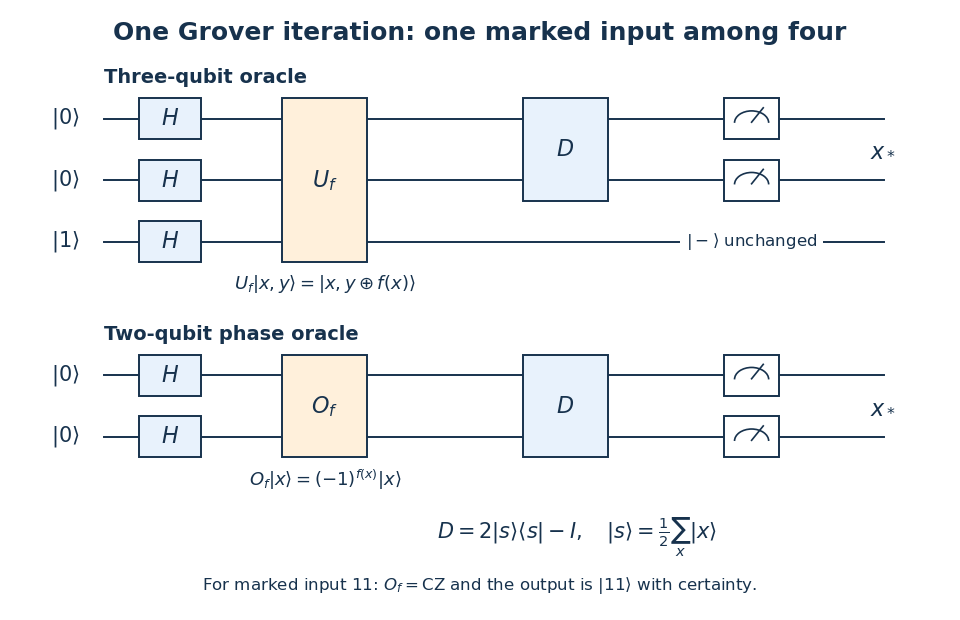
Let and let be one only at the marked input. A three-qubit implementation of Grover's algorithm starts with , applies a Hadamard gate to each qubit, queries the reversible quantum oracle , applies the Grover diffusion operator to the first two qubits, and measures those two qubits in the computational basis. Here . The full three-wire quantum circuit is the composition
Figure 1.
Three- and two-qubit implementations of Grover's algorithm for four inputs
. Details.
Here . Since , phase kickback gives . The third qubit remains separable and unchanged. A direct marked-state phase oracle therefore replaces the three-qubit query using only two qubits:
For the explicit choice only at , is a Controlled-Z gate. Immediately after it,
The mean of these four probability amplitudes is . The Grover diffusion operator maps each probability amplitude to . The three unmarked probability amplitudes become zero and the marked one becomes one. A single query consequently finds with probability one.
A gate-level implementation of is . Up to an irrelevant global phase, it is . For any other chosen marked word, conjugate the Controlled-Z gate by Pauli X gates on precisely the positions where the marked word has a zero.
The five DiVincenzo criteria are: a scalable collection of well-characterized qubits; preparation in a known fiducial quantum state; relevant coherence times long compared with quantum gate times; a universal quantum gate set; and qubit-specific quantum measurement. The criterion is useful control of the whole computation, including errors, rather than merely observing two resolved levels.[ref]
For trapped ions, the implementation is:
For trapped neutral atoms, the corresponding implementation is:
Thus neither platform is forbidden from meeting a criterion in principle. Weak neutral-ground-state interactions make entangling control harder, but claiming that trapped neutral atoms cannot implement a universal quantum gate set would be false. Gate-model quantum algorithms using Rydberg blockade had already been demonstrated in a programmable neutral-atom processor by 2022.[ref]
Zero-point fields are the irreducible electromagnetic field fluctuations in the vacuum state. Each normal mode has ground energy . Although in the vacuum state, d gives . These are quantum fluctuations, not a classical random coherent field with a known instantaneous value.
Two consequences are the Lamb shift, where coupling to the quantized electromagnetic field changes atomic energy levels, and spontaneous emission, where an excited chemical atom can emit a photon into an initially empty normal mode. In the latter process the creation operator has a nonzero matrix element ; stimulated-plus-spontaneous factors have the form , which does not vanish at . Descriptions splitting spontaneous emission into vacuum fluctuations and radiation reaction depend on operator-ordering conventions; the measurable total rate does not. Zero-point fields do not mean that the vacuum state contains a nonzero mean photon number.
For the normalized coherent state, and . The dimensionless electric field and magnetic field optical quadratures consequently have expectation values
The physical electric field and magnetic field strengths have the corresponding proportionality factors and mode functions. In free evolution replace by to recover the classical oscillation.
Expanding the squared operators cancels the and terms:
On the other hand, . Hence
The difference is the sum of the variances, not an extra mean field. Indeed , independent of . The commutator requires , and the coherent state attains equality. The residual two units are the vacuum fluctuations of the two optical quadratures.
The number operator is . The number state expansion gives by shifting the summation index; taking the adjoint gives . Thus the expectation value is
For the second moment, use :
Its expectation value in the coherent state is . Therefore
The variance equals the mean, exactly as for the Poisson distribution found in b. For the fractional standard deviation is , the usual photon shot noise scaling. For the vacuum state, both the mean photon number and its variance vanish; this does not imply zero optical quadrature fluctuations. At the fractional fluctuation is undefined.
Set and . Their commutator is
It commutes with both operators, so the stated Baker--Campbell--Hausdorff formula terminates:
In particular . Expanding the remaining exponential and using gives the number state expansion
The orthonormality of the number states gives
This is a Poisson distribution with parameter . Its probabilities sum to . The phase of affects the coherent state's relative probability amplitudes but not its photon number probabilities. At the distribution is concentrated at .

Pinned article: Introduction to the OurBigBook Project

Welcome to the OurBigBook Project! Our goal is to create the perfect publishing platform for STEM subjects, and get university-level students to write the best free STEM tutorials ever.
Everyone is welcome to create an account and play with the site: ourbigbook.com/go/register. We belive that students themselves can write amazing tutorials, but teachers are welcome too. You can write about anything you want, it doesn't have to be STEM or even educational. Silly test content is very welcome and you won't be penalized in any way. Just keep it legal!
We have two killer features:
  1. topics: topics group articles by different users with the same title, e.g. here is the topic for the "Fundamental Theorem of Calculus" ourbigbook.com/go/topic/fundamental-theorem-of-calculus
    Articles of different users are sorted by upvote within each article page. This feature is a bit like:
    • a Wikipedia where each user can have their own version of each article
    • a Q&A website like Stack Overflow, where multiple people can give their views on a given topic, and the best ones are sorted by upvote. Except you don't need to wait for someone to ask first, and any topic goes, no matter how narrow or broad
    This feature makes it possible for readers to find better explanations of any topic created by other writers. And it allows writers to create an explanation in a place that readers might actually find it.
    Figure 1.
    Screenshot of the "Derivative" topic page
    . View it live at: ourbigbook.com/go/topic/derivative
  2. local editing: you can store all your personal knowledge base content locally in a plaintext markup format that can be edited locally and published either:
    This way you can be sure that even if OurBigBook.com were to go down one day (which we have no plans to do as it is quite cheap to host!), your content will still be perfectly readable as a static site.
    Figure 5. . You can also edit articles on the Web editor without installing anything locally.
    Video 3.
    Edit locally and publish demo
    . Source. This shows editing OurBigBook Markup and publishing it using the Visual Studio Code extension.
  3. https://raw.githubusercontent.com/ourbigbook/ourbigbook-media/master/feature/x/hilbert-space-arrow.png
  4. Infinitely deep tables of contents:
    Figure 6.
    Dynamic article tree with infinitely deep table of contents
    .
    Descendant pages can also show up as toplevel e.g.: ourbigbook.com/cirosantilli/chordate-subclade
All our software is open source and hosted at: github.com/ourbigbook/ourbigbook
Further documentation can be found at: docs.ourbigbook.com
Feel free to reach our to us for any help or suggestions: docs.ourbigbook.com/#contact