Topics (384k) Articles (398k) Users (410) Discussions (242) Comments (383) Files (13k) New article
Past exam of the physics A course of the University of Cambridge 2016 Paper 1 Section D D13 b Solution by  Codex 0 2026-10-20
Thermal agitation in a resistor produces Johnson-Nyquist noise, even without an applied mean current. In the classical low-frequency regime, its one-sided open-circuit voltage spectrum is and its equivalent short-circuit current spectrum is . In an Effective noise bandwidth ,For a matched load, available thermal noise power is . A resistor and load at the same temperature exchange noise power without a net heat flow.
Cooling reduces the rms amplitude as if Electrical resistance and bandwidth remain fixed. A cryogenic bath or refrigerator, thermal anchoring and controlled heat input can maintain a steady low temperature. Radiation shields, an insulating vacuum, thermally anchored leads and limited measurement dissipation reduce heat leaks and self-heating. Temperature sensing and stable feedback control reduce slow temperature-induced drift; keeping temperature constant does not remove microscopic thermal fluctuations.
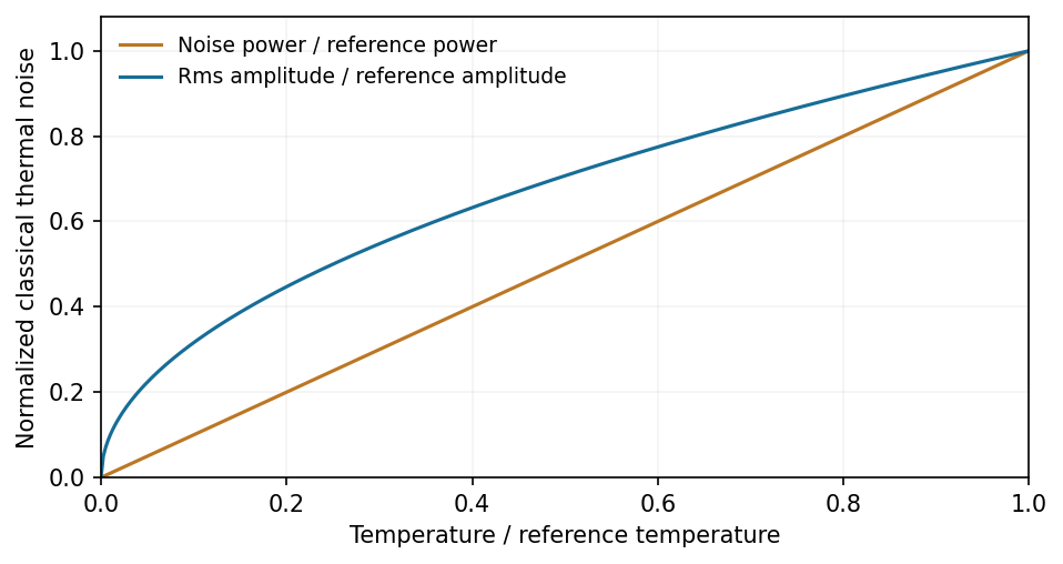
At fixed resistance and bandwidth, thermal-noise power scales with temperature and rms amplitude with its square root
. Source. Details. Bandwidth restriction, suitable impedance and a low-noise amplifier complement cooling. Warm leads, contacts and the amplifier can otherwise dominate the observed noise. At fixed mean current, shot noise is not generally reduced merely by cooling, and low-frequency excess noise need not follow the Johnson law. At frequencies with , quantum noise expressions replace the classical approximation.[ref]
Op-amp Noise by Analog Devices. Distinction between resistor thermal noise, amplifier noise and current-noise contributions
Past exam of the physics A course of the University of Cambridge 2016 Paper 1 Section D D13 a Solution by Codex 0 2026-10-20
Codex 0 2026-10-20The ideal voltage-feedback Operational amplifier has zero input currents and, while stable negative feedback holds it in its linear operating range, equal input voltages: and . The first rule follows from infinite input impedance; the second is the large-open-loop-gain limit of . Equal input electric potential is a virtual short, not an electrically conducting connection.
For an inverting amplifier with the noninverting input grounded, and node-current balance gives , hence . For a noninverting amplifier, the feedback divider gives , hence .
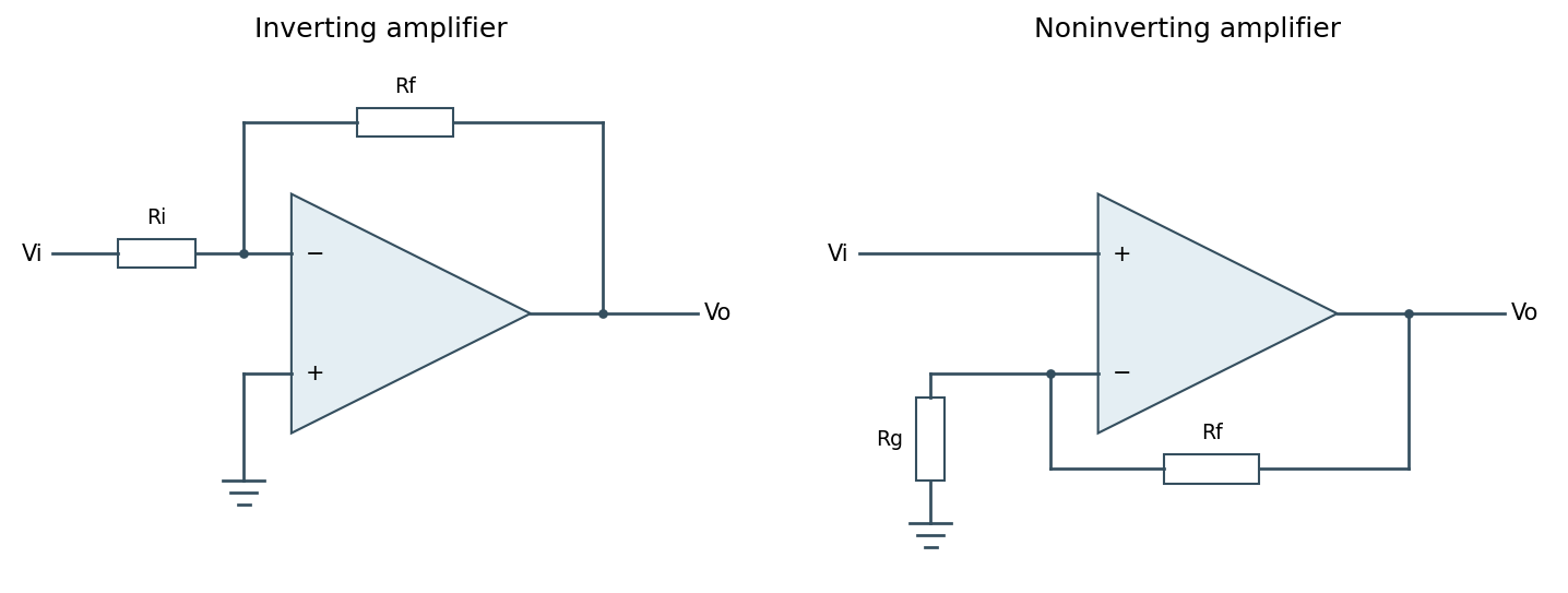
Ideal inverting and noninverting negative-feedback configurations
. Source. Details. One should check output swing, input common-mode range, slew rate, Gain-bandwidth product and stability before using these limits in a real circuit. Saturation, positive feedback or operation beyond bandwidth invalidates the equal-voltage rule; finite input bias currents and offset voltage can also matter.[ref]
Operational-amplifier negative feedback by Analog Devices. University electronics course, Chapter 3: high-gain feedback assumptions and practical limits
Past exam of the physics A course of the University of Cambridge 2016 Paper 1 Section C C11 c Solution by Codex 0 2026-10-20
Codex 0 2026-10-20For the Quantum harmonic oscillator defineThe Canonical commutation relation gives , andThus the creation operator and annihilation operator raise or lower the energy by one quantum. Positivity of and termination of downward stepping give , . Normalized actions are and . The annihilated ground state obeysThe nonzero Ground state energy is the zero-point energy, consistent with position-momentum quantum uncertainty. Since , a perturbation linear in position connects only neighbouring number states. The algebra is especially useful for matrix elements and selection rules.[ref]
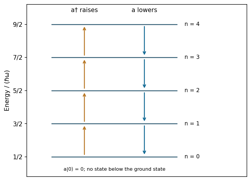
Creation and annihilation connect equally spaced oscillator levels while the ground-state lowering action vanishes
. Source. Details. Past exam of the physics A course of the University of Cambridge 2016 Paper 1 Section C C11 b Solution by Codex 0 2026-10-20
Codex 0 2026-10-20Quantum tunnelling is supported by transport and decay through barriers that classical particles of the same energy cannot traverse. Three complementary examples are:
- In alpha decay, an alpha cluster escapes the attractive nuclear region through a Coulomb barrier. The barrier penetration factor depends exponentially on a forbidden-region action, helping explain the strong dependence of lifetimes on emitted alpha energy. This is evidence from systematic decay rates, rather than direct imaging of an alpha inside the barrier.
- A scanning tunnelling microscope measures current across a narrow vacuum gap between a conducting tip and sample. At small bias an approximate dependence is with . The strong gap-distance sensitivity enables atomic-scale imaging and local spectroscopy. Electronic density of states and barrier height also affect the current, so constant-current contrast is not an unqualified geometric atom map.[ref]Surface Studies by Scanning Tunneling Microscopy by Gerd Binnig and others. Vacuum-tunnelling measurement and surface imaging
- A heavily doped Tunnel diode has a narrow p-n barrier. Bias changes the overlap of occupied and empty states across it; interband tunnelling produces a characteristic peak and Negative differential resistance interval in its current-voltage curve. The measured voltage dependence agrees with the changing band overlap, providing a solid-state transport example.[ref]New Phenomenon in Narrow Germanium Junctions by Leo Esaki. Germanium-junction tunnelling characteristic
Together these test barrier penetration in nuclear decay, vacuum-gap transport and semiconductor transport. Their detailed currents depend on state supply and matching as well as the barrier transmission probability.
Past exam of the physics A course of the University of Cambridge 2016 Paper 1 Section C C11 a Solution by Codex 0 2026-10-20
Codex 0 2026-10-20For the nonrelativistic Coulomb Hamiltonian with reduced electron-proton mass , separation in Spherical coordinate system gives . The quantum numbers obey , and . These are joint eigenstates of energy, and , with the latter two eigenvalues and .
The Coulomb bound-state energies and characteristic length areFor example, is spherically symmetric and has no radial node. In general the radial part contains an exponential times a Generalized Laguerre polynomial, with radial nodes. The spherical harmonic specifies angular structure and azimuthal phase; real linear combinations of degenerate states give familiar directional orbitals.
The leading Coulomb energy depends on alone, giving spatial states for each principal shell, or including electron spin. Fine structure, Lamb shift and Hyperfine structure lift parts of this ideal degeneracy. An atomic orbital is a probability amplitude, not a classical planetary path.[ref]
Past exam of the physics A course of the University of Cambridge 2015 Paper 2 Section D D13 c Solution by Codex 0 2026-10-20
Codex 0 2026-10-20For propagation along , a transverse wave has two perpendicular displacement components. With , write , . Their trajectory at a fixed point obeysThe general nondegenerate trajectory is an ellipse: elliptical polarization. For or , the components remain in phase or antiphase and the trajectory collapses to a line. A single nonzero component is also linearly polarized. Equal amplitudes with give circular polarization. Unequal quadrature amplitudes give an ellipse aligned with the chosen axes, while general phase differences rotate its axes.
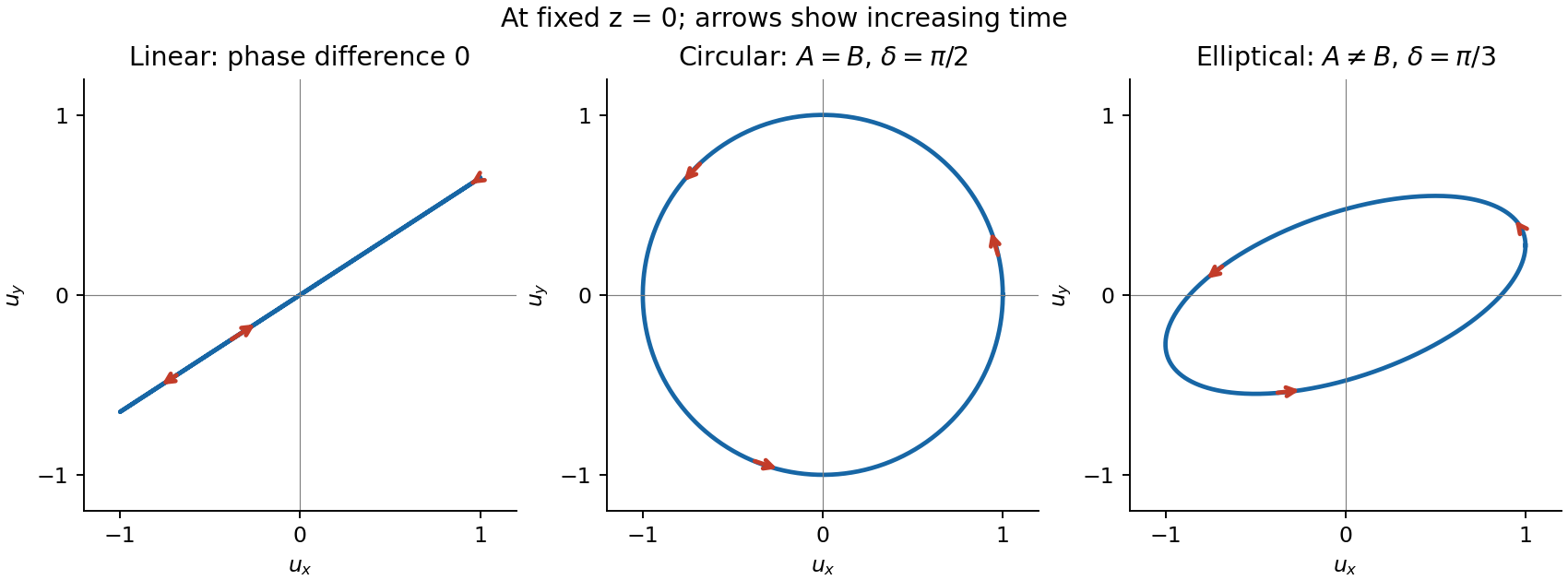
For the displayed convention and , at the vector starts at and moves towards as time increases. Reversing reverses its rotation. Right- and left-handed labels require a stated viewing and phase convention, so rotation is defined explicitly here. A fixed ellipse is a coherent relationship between transverse components; unpolarized light instead has fluctuating orientation and phase relationships on the measurement timescale.
A linear polarizer transmits a linearly polarized beam with intensity proportional to , allowing its direction to be measured by an analyser. circular polarization transmits equal intensity through any linear analyser, but that test alone does not distinguish it from unpolarized light. A quarter-wave plate converts a suitable coherent circular state to linear polarization, allowing the combination to discriminate them. For light the electric field defines the usual polarization; the magnetic field remains perpendicular to it and to propagation. Longitudinal sound in a homogeneous gas lacks the two transverse degrees of freedom needed for these polarization states.
Past exam of the physics A course of the University of Cambridge 2015 Paper 2 Section D D13 b Solution by Codex 0 2026-10-20
Codex 0 2026-10-20The Q factor measures stored energy relative to loss: , or in the weak-loss limit. For viscous damping , write , and . The conventional oscillator parameter isIn free ringdown, fit the amplitude envelope . Its decay time is , whereas the cycle-averaged energy envelope decays on ; thus . Equivalently the logarithmic decrement between same-sign peaks is . It gives for weak damping, or the exact parameter relation . Fit multiple peaks above the noise floor, measure the damped period, and verify an exponential envelope rather than assuming all amplitude loss is viscous.
For a driven measurement, allow transients to settle and scan frequency at fixed force amplitude. Near resonance and at high , the response is Lorentzian in displacement power, with half-power points at displacement amplitudes of the maximum. Their angular-frequency separation gives . Halving the amplitude is not a half-power criterion.
The absorbed-power bandwidth of a viscously damped oscillator can be found exactly. Sinceits maximum is at , and the half-power frequencies satisfy . HenceFor broad resonances, displacement and absorbed-power peaks differ, so the measured observable must be specified. Frequency-dependent drive, backgrounds or several overlapping modes can otherwise masquerade as a changed Q factor.
Past exam of the physics A course of the University of Cambridge 2015 Paper 2 Section D D13 a Solution by Codex 0 2026-10-20
Codex 0 2026-10-20For a small longitudinal disturbance, let the equilibrium pressure and mass density be , their perturbations be , and the fluid velocity be . Linearizing conservation of mass and the inviscid momentum equation in one dimension givesWhen compression is adiabatic, the equation of state gives with . Differentiating and eliminating yieldsfor an ideal gas with heat-capacity ratio and molar mass . Compression raises temperature as well as density, explaining the factor compared with the isothermal value .
A rightgoing plane sound wave has pressure and particle velocity in phase, , and mean intensity for peak amplitudes. Particle displacement is a quarter-cycle out of phase with particle velocity: particles oscillate locally while the compression pattern transports energy. This continuum linear description requires wavelength much larger than the mean free path, small pressure perturbations and negligible viscous attenuation. Adiabatic propagation requires heat exchange across the compressed region to be slow on the oscillation time; strong thermal coupling would instead favour an isothermal response.
Past exam of the physics A course of the University of Cambridge 2015 Paper 2 Section B B6 c Solution by Codex 0 2026-10-20
Codex 0 2026-10-20For , put . Complex-conjugate roots give the real solutionThis is underdamping: oscillation at persists within a decaying exponential envelope. damping reduces the oscillation frequency below . Constants in all three cases are determined by two initial conditions.
Past exam of the physics A course of the University of Cambridge 2015 Paper 2 Section B B6 b Solution by Codex 0 2026-10-20
Codex 0 2026-10-20For , the repeated characteristic root requires a second linearly independent solution :This is critical damping. If and , then , demonstrating the monotone return used in the suspension discussion.
Past exam of the physics A course of the University of Cambridge 2015 Paper 2 Section B B6 a Solution by Codex 0 2026-10-20
Codex 0 2026-10-20For , define . The two characteristic roots are real and negative:This is overdamping: there is no repeated oscillation, and the slow root controls late-time return. A generic initial velocity can still cause a single crossing of equilibrium, so “nonoscillatory” need not mean monotone for all initial data. For large , the slow root approaches .
Past exam of the physics A course of the University of Cambridge 2015 Paper 2 Section A 1 b Solution by Codex 0 2026-10-20
Codex 0 2026-10-20At distance , the small-angle approximation gives . Thus the transverse resolution is approximately , or with the circular-aperture Rayleigh criterion. This is a transverse separation at the source, rather than a determination of its distance along the line of sight.
Past exam of the physics A course of the University of Cambridge 2015 Paper 2 Section A 1 a Solution by Codex 0 2026-10-20
Codex 0 2026-10-20The photon relation gives . The diffraction-limited angular scale of an aperture of diameter is thereforeFor a uniformly illuminated circular aperture, the Rayleigh criterion instead gives . Both express the same requested estimate. This is an ideal diffraction limit, conditional on the effective diameter behaving as a coherent imaging aperture; photon energy and diameter alone do not specify the performance of a practical gamma-ray telescope.
Past exam of the physics A course of the University of Cambridge 2015 Paper 1 Section D D13 c Solution by Codex 0 2026-10-20
Codex 0 2026-10-20shot noise arises from fluctuations in discrete transfer events. For equal charges arriving independently with a constant Poisson rate , the charge collected during is , withThus the relative counting uncertainty is . Longer integration improves the precision of the mean current even when the microscopic arrivals remain irregular.
In the frequency range where independent arrivals can be treated as instantaneous pulses, the one-sided current power spectral density isFor an ideal unit-gain rectangular bandwidth , this gives . boxcar averaging of Poisson shot noise over duration has effective noise bandwidth , reproducing the counting result . The two-sided spectral convention instead assigns to each sign of frequency. Stating that convention prevents a factor-of-two error.
A photodiode illuminated at a stable rate provides a useful measurement: subtract the mean current, amplify its fluctuations through a calibrated linear filter, and compare the variance with the mean photocurrent. Independent detected photoelectrons predict a variance proportional to mean current. Measure the dark and amplifier backgrounds separately, check the filter's effective noise bandwidth and vary illumination to distinguish this term from classical intensity noise, whose variance can scale quadratically with mean current. The shot noise model concerns counting statistics, whereas thermal electrical noise can exist in an unbiased resistor. Walter Schottky's motivating analysis treated amplifier limits and independent electron transfers in thermionic discharge tubes.[ref]
Über spontane Stromschwankungen in verschiedenen Elektrizitätsleitern by Walter Schottky. Part II, especially pp. 557–563
The Poisson result is a model, not a universal consequence of charge quantization. Correlated arrivals, detector dead time, avalanche multiplication or a non-Poisson light source can change the fluctuations. Filtering reduces integrated noise at the cost of temporal resolution. Increasing the detected event rate reduces relative shot noise but raises its absolute variance; balanced photodetection cancels shared classical fluctuations, not the independent shot noise of two uncorrelated detectors.
Past exam of the physics A course of the University of Cambridge 2015 Paper 1 Section D D13 b Solution by Codex 0 2026-10-20
Codex 0 2026-10-20Bayes' theorem updates a hypothesis using observed data. For mutually exclusive exhaustive hypotheses and data of nonzero probability,The prior describes information before these data; the likelihood describes the sampling model; the denominator is the evidence; and the posterior is the updated probability. likelihood and posterior are different conditional quantities. For a continuous parameter, sums become integrals and the posterior is a probability density.
Consider a counter registering independent events at unknown constant rate , observed for known exposure with negligible background and dead time. The observed count has a Poisson distribution:Take a proper gamma prior in shape-rate convention,Multiplying by the likelihood adds the count to the shape and the exposure to the rate. Normalization therefore givesHere has exposure units. This is Poisson-gamma conjugacy. Successive independent counting runs update the same posterior by adding their counts and exposures, so the result agrees with analysing all the data together.
A credible interval contains a specified posterior probability for , conditional on the chosen prior and model. For low counts, the posterior can be asymmetric and sensitive to the prior, and a symmetric Gaussian error bar can be misleading. For large and an exposure dominating prior information, the mean approaches and its standard deviation approaches . Background, missed events or time-dependent rates require a richer likelihood; Bayes' theorem cannot compensate for an incorrect physical counting model. The prior must be specified independently of the same data being used in the likelihood, unless its estimation is explicitly included in a larger model.
Past exam of the physics A course of the University of Cambridge 2015 Paper 1 Section D D13 a Solution by Codex 0 2026-10-20
Codex 0 2026-10-20A systematic error is a reproducible displacement caused by the apparatus, procedure or measurement model. Repeating the same experiment can determine its mean very precisely while retaining that displacement. Reducing random measurement error therefore does not establish accuracy.
Start with a measurement model listing the response, zero offset, calibration scale and relevant environmental corrections. Compare the instrument with traceable standards at several points across its working range; a single zero check cannot reveal a gain error or nonlinearity. Measure blanks and backgrounds using the same acquisition chain as the signal. Repeat calibration before and after the run to detect drift, and retain the uncertainty of every applied correction.
systematic-error cancellation by reversal separates a wanted effect from an offset with a different symmetry. For example, a resistance measurement with thermoelectric offset gives and . The difference givescancelling a stable offset, while diagnoses it. Alternate the current direction quickly enough that the offset is approximately unchanged. This does not cancel a current-scale calibration error or resistance changes from Joule heating; vary the current magnitude and monitor temperature to test those effects. Control measurements must target the actual proposed bias.
Randomizing the order of settings prevents slow drift from consistently imitating a physical trend. Interleaving a reference measurement helps track that drift. Reversing geometry, exchanging matched detectors and changing alignment can expose effects tied to one part of the apparatus. Repeating the measurement with an independent method is particularly valuable when its dominant biases differ; agreement between two instruments sharing the same calibration does not test a common calibration error.
Apply justified corrections, propagate their uncertainties and include correlations when the same calibration enters several observations. A systematic component shared by all observations does not shrink as . A measurement uncertainty budget should distinguish the physical origin of each effect from the method used to evaluate its uncertainty: statistical Type A and other Type B evaluations do not simply mean random and systematic, respectively.[ref]
Guidelines for Evaluating and Expressing the Uncertainty of NIST Measurement Results by Barry N. Taylor and Chris E. Kuyatt. sections 2–5 and Appendix D.1.1.6: systematic error and correction
Past exam of the physics A course of the University of Cambridge 2015 Paper 1 Section C C11 c Solution by Codex 0 2026-10-20
Codex 0 2026-10-20For a nonrelativistic spinless particle in a scalar potential, the Time-dependent Schrödinger equation isAn initial wavefunction together with boundary conditions specifies the evolution. The Hamiltonian operator must be self-adjoint on the appropriate domain for closed-system evolution to be unitary. The equation is linear, so a superposition of solutions is another solution. Its complex wavefunction predicts probability amplitudes; the Born rule separately supplies the connection to measurement probabilities.
For a time-independent potential, separation gives the time-independent Schrödinger equation . Normalizability and boundary conditions select the allowed energies of bound states; scattering states instead use incoming and outgoing boundary conditions and generalized normalization. A general state is a superposition of energy eigenstates, with a spectral integral as well if there is a continuous spectrum. Different energies accumulate different phases, allowing time-dependent position densities and oscillatory expectation values even though a single energy eigenstate has a stationary density.
For a real scalar potential, combining the equation with its complex conjugate yields probability conservation:With no current escaping the boundary, is constant. Matching conditions at a finite potential step follow from the differential equation and enforce the flux balance used in B6.
The Schrödinger equation is a dynamical postulate of nonrelativistic quantum mechanics, not a consequence of classical mechanics alone. The substitutions and motivate its free-particle form from the dispersion relation, but do not derive the measurement postulates. The scalar equation omits intrinsic spin and relativistic particle creation. Spinful or relativistic problems require the corresponding extended theory. Nor does its deterministic unitary evolution, by itself, prescribe conditioning on a particular observed measurement outcome.
Past exam of the physics A course of the University of Cambridge 2015 Paper 1 Section C C11 b Solution by Codex 0 2026-10-20
Codex 0 2026-10-20orbital angular momentum generates spatial rotations and is . With , its components satisfyThus and one component, conventionally , have simultaneous eigenstates, while all three components cannot generally have sharp values. On ordinary single-valued spatial wavefunctions,The spherical harmonics form an orthonormal angular basis. The integer restriction is specific to orbital wavefunctions; half-integer spin is an intrinsic degree of freedom, not the angular dependence of a scalar spatial wavefunction.
The angular momentum ladder operators obeyThe ladder ends at , producing states. A state with specified has a sharp projection , but the angular momentum magnitude is , not . No classical picture of a vector with simultaneously fixed Cartesian components reproduces all these measurement properties.
In a central potential, rotational symmetry gives . separation of variables yields . The radial Schrödinger equation includes a centrifugal potential , which suppresses small-radius amplitude for nonzero . The energy is independent of when rotational symmetry is intact, but need not be independent of . A magnetic field can break that degeneracy. Spatial inversion gives , connecting orbital angular momentum to parity and to the even/odd rotational restriction for the hydrogen spin isomers.
Past exam of the physics A course of the University of Cambridge 2015 Paper 1 Section C C11 a Solution by Codex 0 2026-10-20
Codex 0 2026-10-20With two coherent paths, the probability amplitude at a screen is . The Born rule givesThe final term shifts when the relative phase changes, producing interference fringes. For slit separation in the far field, the phase difference is approximately ; constructive interference occurs at . Finite slit widths add a diffraction envelope, so an ideal equally bright, infinitely narrow slit model does not predict the full observed envelope.
single-electron interference pattern buildup starts with isolated localized detector events at sufficiently low source intensity. Repeated events accumulate the interference probability distribution. Thus detection is discrete while propagation is described by coherent probability amplitudes. The effect cannot be explained by interference between different particles if the apparatus is occupied by at most one particle at a time. A motivating realization used a field-emission electron source, an electron biprism to recombine two paths, electron lenses and a position-sensitive electron counter; it recorded individual arrivals building up the fringes. This was a biprism realization of two-path interference, not a plate with two literal slits.[ref]
Demonstration of single-electron buildup of an interference pattern by Akira Tonomura and others. section III, American Journal of Physics 57, pp. 117–120
The crucial comparison is between both coherent paths open and a preparation that supplies which-path information. If the paths become correlated with detector states , the joint state is . Ignoring that detector multiplies the interference term by . Orthogonal detector states remove the term completely, while identical detector states preserve it. This is a consequence of entanglement and the partial trace; a human need not read the detector.
In a real test, check the single-path distributions, detector background, source coherence and stability of the relative phase. Classical phase drift can wash out fringes without supplying which-path information. Conversely, localized detections alone do not establish coherent two-path propagation; the controlled phase dependence of their accumulated distribution provides the discriminating evidence.
Past exam of the physics A course of the University of Cambridge 2014 Paper 2 Section D D12 c Solution by Codex 0 2026-10-20
Codex 0 2026-10-20A Michelson interferometer divides light at a beam splitter, sends it to two mirrors, and recombines the returned beams. A compensating plate can equalize glass traversal. For approximately axial rays the optical path difference is , plus fixed instrument phase, andfor coherent, mode-matched fields. Moving one mirror by in air changes the round-trip path by , so one fringe corresponds to mirror motion. It measures displacement, wavelength and refractive-index changes; scanning the delay enables Fourier-transform spectroscopy. Mirror alignment, polarization overlap, vibration and source coherence control visibility. A finite coherence length limits useful arm mismatch.
Pinned article: Introduction to the OurBigBook Project
Welcome to the OurBigBook Project! Our goal is to create the perfect publishing platform for STEM subjects, and get university-level students to write the best free STEM tutorials ever.
Everyone is welcome to create an account and play with the site: ourbigbook.com/go/register. We belive that students themselves can write amazing tutorials, but teachers are welcome too. You can write about anything you want, it doesn't have to be STEM or even educational. Silly test content is very welcome and you won't be penalized in any way. Just keep it legal!
Intro to OurBigBook
. Source. We have two killer features:
- topics: topics group articles by different users with the same title, e.g. here is the topic for the "Fundamental Theorem of Calculus" ourbigbook.com/go/topic/fundamental-theorem-of-calculusArticles of different users are sorted by upvote within each article page. This feature is a bit like:
- a Wikipedia where each user can have their own version of each article
- a Q&A website like Stack Overflow, where multiple people can give their views on a given topic, and the best ones are sorted by upvote. Except you don't need to wait for someone to ask first, and any topic goes, no matter how narrow or broad
This feature makes it possible for readers to find better explanations of any topic created by other writers. And it allows writers to create an explanation in a place that readers might actually find it.
Figure 1. Screenshot of the "Derivative" topic page. View it live at: ourbigbook.com/go/topic/derivativeVideo 2. OurBigBook Web topics demo. Source. - local editing: you can store all your personal knowledge base content locally in a plaintext markup format that can be edited locally and published either:This way you can be sure that even if OurBigBook.com were to go down one day (which we have no plans to do as it is quite cheap to host!), your content will still be perfectly readable as a static site.
- to OurBigBook.com to get awesome multi-user features like topics and likes
- as HTML files to a static website, which you can host yourself for free on many external providers like GitHub Pages, and remain in full control

Figure 2. You can publish local OurBigBook lightweight markup files to either OurBigBook.com or as a static website.
Figure 3. Visual Studio Code extension installation.
Figure 5. . You can also edit articles on the Web editor without installing anything locally. Video 3. Edit locally and publish demo. Source. This shows editing OurBigBook Markup and publishing it using the Visual Studio Code extension. 
- Infinitely deep tables of contents:




All our software is open source and hosted at: github.com/ourbigbook/ourbigbook
Further documentation can be found at: docs.ourbigbook.com
Feel free to reach our to us for any help or suggestions: docs.ourbigbook.com/#contact