Phase folding of a light curve collects samples at equal trial phase. Consider a noiseless illustrative pulsar with one pulse every $P=1.4\mathrm{s}$ and arrival times $t_n=nP$, after pulsar dedispersion. At $P_{\mathrm{trial}}=P$, all arrivals fold to one phase. But $P/2$ also puts all arrivals at one phase: folding discarded the fact that alternate proposed cycles contain no pulse. At $2P$, the arrivals instead occupy two phases, $0$ and $1/2$. Thus a sharp folded profile alone need not identify the fundamental period.

Check the original time sequence, adjacent arrival intervals and pulse occupancy as well as the folded profile. With $N$ arrivals and a slightly wrong trial period, the unwrapped drift isFor $N=100$ and $P_{\mathrm{trial}}=1.401\mathrm{s}$, this is about $-0.07066$ cycle. Splitting the observation into early and late pieces reveals the drift that one full folded average can blur. Separately, regular discrete sampling can create aliasing: observing at a spacing comparable with the pulse width can miss narrow pulses even when the recurrence period is much longer. Neither this toy exercise nor one sharp profile replaces time-standard calibration and propagation corrections.

A radio wave traversing a dilute cold plasma has a group velocity that depends on its frequency. In the ideal unmagnetized limit, the dispersion relation is ${\omega }^2=c^2{k}^2+{\omega }_p^2$, where ${\omega }_p$ is the angular plasma frequency. For $\omega \gg {\omega }_p$, differentiate to obtain $v_g=c\sqrt{1-{\omega }_p^2/{\omega }^2}$, then expand $1/v_g$ to first order. The excess travel time over a vacuum path isHere $f=\omega /(2\pi )$ is ordinary frequency, $e$ is the magnitude of the elementary charge, $m_e$ is the electron mass, ${ϵ}_0$ is the vacuum permittivity, $n_e$ is electron number density, and $c$ is the speed of light. This approximation neglects magnetic corrections, collisions and multipath scattering; its positive sign means lower frequencies arrive later.

Jocelyn Bell Burnell helped build Antony Hewish's radio telescope for finding compact sources through interplanetary scintillation in the solar wind. Operating it and inspecting its chart recorder output in 1967, she recognized an unusual recurring trace, checked earlier charts, and obtained fast recordings resolving pulses in late November. Her observation, recognition and persistent analysis were indispensable.^[ref]

The 1968 paper by Antony Hewish, Jocelyn Bell Burnell (bylined S. J. Bell), J. D. H. Pilkington, P. F. Scott and R. A. Collins reported $1.337\mathrm{s}$ spacing and proposed compact-star oscillations. Its radio telescope had 2,048 full-wave dipole antennas in sixteen rows. Four receivers selected declinations; two array halves formed an east-west interferometer. The $81.5\mathrm{MHz}$ receivers passed $1\mathrm{MHz}$. Observations used $0.05\mathrm{s}$ receiver time constant and Rapidigraph chart recorder with $0.03\mathrm{s}$ time constant; radio second pips calibrated timing.^[ref]

Antony Hewish checked sidereal time recurrence. Jocelyn Bell Burnell recalls that P. F. Scott and R. A. Collins reproduced the pulses with another telescope and receivers, while J. D. H. Pilkington measured pulsar dispersion delay: independent checks of instrument independence and intervening plasma.^[ref]

A useful numerical comparison uses the approximate sidereal time day of $1436.07\min$. Relative to a $1440\min$ schedule, the same sky direction transits about $3.93\min$ earlier each day, or $39.3\min$ after ten days. This compares successive passages through the receiving beam; it is a different clock from the roughly $1.3\mathrm{s}$ pulse spacing within one passage. Sky recurrence alone cannot rule out every transmitter or reflection, and pulsar dispersion delay alone does not uniquely establish an emission mechanism. Their strength lies in independent constraints agreeing.

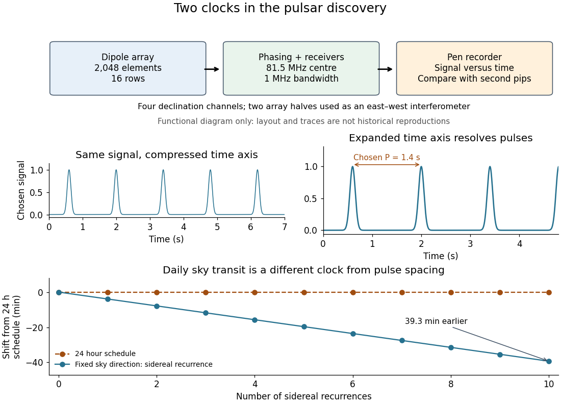
The discovery lesson is that an unexpected signal must survive changes of readout, instrument and observing date. Increasing chart recorder speed exposed structure hidden in a compressed trace; it did not make the source begin pulsing. The pulsar interpretation now separates the rotating clock, beam geometry, pulsar magnetosphere emission and pulsar dispersion delay. The initial observation established periodic arrival, not a direct measurement of the neutron star's surface motion or radius.

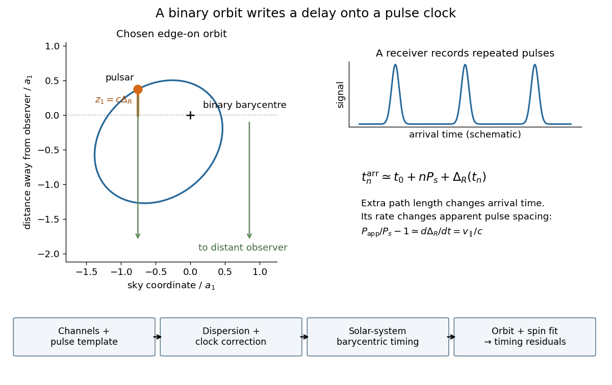
A binary pulsar is a pulsar in a binary star: the companion's gravity changes the emitting neutron star's motion and hence its pulse arrival times. The companion need not itself be a detectable pulsar. Pulsar timing turns that motion into a measurable orbit, making the system useful for stellar mass determination and tests of general relativity.

The mature experiment uses channel-template comparison, pulsar dedispersion, GPS clock-offset transfer, Solar system barycenter corrections and connected pulse counts.^[ref]

For a geometric illustration, let a perfectly uniform source emit pulse $n$ at $t_n=t_0+n{P}_s$, with spin period $P_s$, and let $z_1$ increase away from the observer. At leading order in orbital velocity divided by the speed of light, an extra path length $z_1$ adds ${\Delta }_R=z_1/c$. Consecutive arrivals then obeyA receding source has $v_{\parallel }>0$ and a longer apparent period. This derivation isolates the geometric Doppler effect; a precision relativistic clock model also needs gravitational redshift and time dilation.

A proteinogenic amino acid represented by R or Arg in protein primary structure. Its amino acid side chain carries predominantly positive electric charge near neutral pH.^[ref]

Trypsin preferentially cleaves after its amino acid residues.

A proteinogenic amino acid represented by K or Lys in protein primary structure. Its amino acid side chain carries predominantly positive electric charge near neutral pH.^[ref]

Trypsin preferentially cleaves after its amino acid residues.

For the prolate spheroid $u^2/a^2+(v^2+w^2)/b^2=1$ with $a>b>0$, intersect the concentric sphere $u^2+v^2+w^2=R^2$. When $b<R<a$, subtraction gives two circles in the perpendicular planesTheir centers lie on the long principal axis and the line through the centers is normal to both planes. At $R=b$ the circles merge into the equator; at $R=a$ they shrink to the two polar vertices. There is no intersection for $R<b$ or $R>a$.

At fixed temperature, the particle count of an isothermal sphere is proportional to ${\rho }_c^{-1/2}f(\xi )$, where $f={\xi }^2{\Psi }^{\prime }$ and $f^{\prime }={\xi }^2{e}^{-\Psi }$. A fixed-mass variation therefore satisfies $\delta {\rho }_c/{\rho }_c=2e^{-\Psi }\delta \xi /{\Psi }^{\prime }$. The boundary density changes by $\delta \rho /\rho =\delta {\rho }_c/{\rho }_c-{\Psi }^{\prime }\delta \xi$. Its first stationary point occurs when the title condition holds. This follows a sequence of equilibria, rather than differentiating the radial profile of one equilibrium. The associated boundary radius obeys $\delta r/r=(1/\xi -e^{-\Psi }/{\Psi }^{\prime })\delta \xi$.

If phase-randomizing collisions form a Poisson process of mean interval ${\tau }_c$, field correlation survives only when no such collision occurs during the delay. Thus its magnitude decays as $e^{-|\tau |/{\tau }_c}$. The Wiener-Khinchin theorem gives the normalized Lorentzian line shapeIts full width at half maximum is $2/{\tau }_c$ in angular frequency or $1/(\pi {\tau }_c)$ in ordinary frequency. A population lifetime is a different time constant: lifetime-limited amplitude decay at half the population rate introduces the familiar factor of two. The definition of the supplied lifetime must therefore accompany any numerical linewidth.

Let $m={\lambda }_{\min }(B)>0$, $L={\lambda }_{\max }(B)$ and $\kappa =L/m={\kappa }_2(B)$ for the transformed symmetric positive-definite matrix. Then preconditioned steepest descent satisfiesThis is a worst-case bound, not necessarily the actual rate. For our scaled example the bound is $(1/50{)}^2=0.0004$, slightly above its computed factor $q_M\approx 0.000384321291$. If the initial transformed error is an eigenvector, exact line search for a positive-definite quadratic removes it in one step, regardless of the full condition number.

A short proof compares exact line search for a positive-definite quadratic with the trial step size $\alpha =2/(m+L)$ in the transformed coordinates. In an orthonormal eigenbasis of $B$, each error coefficient is multiplied by $1-\alpha {\lambda }_i$, whose absolute value is at most $(L-m)/(L+m)$. Summing ${\lambda }_i$ times the squared coefficients bounds the trial energy by the square of this factor. The exact minimizing step size does at least as well. This also explains the terminating case $m=L$: the trial step removes the entire error in one iteration.

In the potential method, an operation's amortized cost is ${\hat{c}}_i=c_i+{\Phi }_i-{\Phi }_{i-1}$. It can exceed or fall below its actual cost $c_i$. The endpoint potentials determine how the total charge compares with the total actual cost.

A function holomorphic outside a disk has a pole of positive integer order $N$ at infinity when its reciprocal-coordinate representative $f(1/w)$ has a pole of that order at $w=0$. Equivalently $f(z)=z^{N}g(1/z)$ with $g$ holomorphic and nonzero at zero. The Laurent series about infinity is interpreted in this coordinate: finitely many positive powers of $z$ form its principal part. For example, $z^N{e}^{1/z}=z^N+z^{N-1}+\cdots$ has a pole of order $N$ at infinity despite its essential singularity at zero.

Consider a teaching extension with two opposite detectors, labelled $+$ and $-$ by fixed laboratory directions, and two preparation states $s=+1,-1$ with equal and opposite nuclear polarization. This is an original two-detector model; the historical Wu experiment used a fixed internal electron counter with reversal.^[ref] Let $C_s>0$ describe the exposure in each state and ${\eta }_d>0$ the stable detection efficiency of detector $d$.

For matched opposite acceptances, write their common mean absolute cosine as $k$. The four expected positive counts areThe same-state ratios each retain the unequal detection efficiencies:Dividing these ratios gives the spin-reversal cross-ratio for beta decay:Both the exposure ratio $C_{+}/C_{-}$ and the detection efficiency ratio ${\eta }_{+}/{\eta }_{-}$ cancel. The positive square root is essential: positive expected counts and $|ϵ|<1$ make $(1+ϵ)/(1-ϵ)$ positive.

For the chosen $a=-0.3$, opposite hemispheres give $k=1/2$, hence $ϵ=-0.15$. Choose $C_{+}=10000$, $C_{-}=8000$, ${\eta }_{+}=0.8$, and ${\eta }_{-}=0.5$, with their common acceptance factor absorbed into $C_s$. The four expected counts in the displayed order are $6800$, $5750$, $7360$, and $3400$. ThusThe first raw detector ratio exceeds one despite negative $ϵ$: detector imbalance can overwhelm the physical directional preference. Reversal separates the stable imbalance from the term that changes sign.

Take boundary data one on a disk of radius $a>0$ and zero outside. The Poisson kernel for the upper half-space gives on the axisThe axis value tends to one at the boundary and behaves as $a^2/(2z^2)$ far away. The boundary data at the circular rim are understood almost everywhere: changing a value on the rim, a set of planar measure zero, leaves the integral unchanged. This does not assert a continuous boundary extension across the jump.

For square-integrable periodic boundary data and the Fourier coefficients used in the Poisson kernel for the unit disk, the displayed identity gives the squared area norm of its Poisson extension $u$. At fixed radius $r$, Parseval's identity givesMultiply by the polar coordinates area element factor $rdr$ and integrate from zero to one. The constant term contributes $\pi |a_0{|}^2/4$, and ${\int }_0^1{r}^{2n+1}dr=1/[2(n+1)]$. Interchanging the nonnegative sum and radial integral is justified by the monotone convergence theorem. The resulting factor $1/(n+1)$ shows how higher angular frequencies contribute less to the interior area norm.

For an independent count with a Poisson distribution of mean $RT$, the rate estimator $N/T$ has variance $R/T$. Its fractional standard deviation is $1/\sqrt{RT}$, so achieving target fractional precision $ϵ$ requires expected count $RT={ϵ}^{-2}$ and exposure $T=1/({ϵ}^{2}R)$.

For independently acquired settings with rates $R_i$, the required total exposure is ${ϵ}^{-2}{\sum }_i{R}_i^{-1}$. Rare settings dominate because they require the same expected count but collect it more slowly. Simultaneous acquisition is a different design, and backgrounds or correlated systematic errors require a different uncertainty calculation.

A material exhibiting piezoelectricity, used in the Curie ionization-current measurement to supply a controlled electric charge.