Topics (384k) Articles (398k) Users (410) Discussions (242) Comments (383) Files (13k) New article
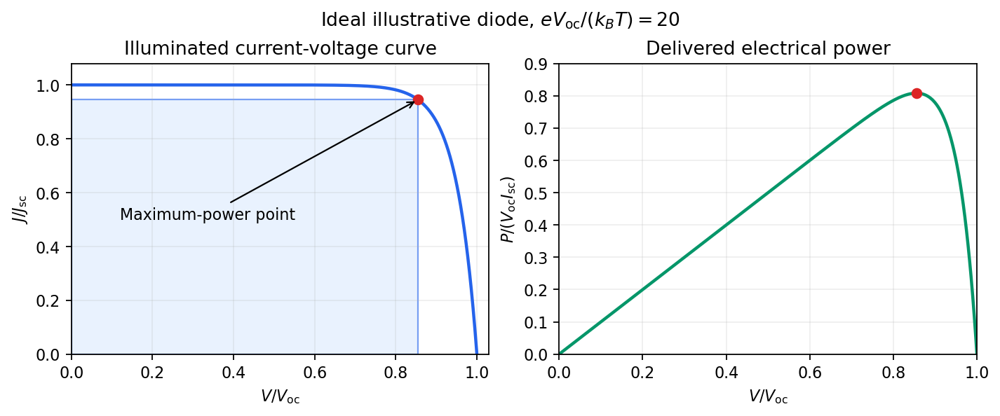
The solar-cell fill factor compares the maximum delivered electrical power with the rectangle formed by the open-circuit electric potential difference and short-circuit electric current. It measures the shape of the illuminated current-voltage characteristic. The conversion efficiency is .
The Shockley-Queisser limit is the radiative conversion-efficiency bound for an ideal single-junction solar cell, with one collected electron-electron hole pair per absorbed above-gap photon, carrier thermalization, and radiative recombination required by the reverse optical process. Photons below the band gap are not absorbed, while excess photon energy above it is thermalized. Maximizing the electrical power over the operating electric potential difference and then the band gap gives a ceiling of roughly thirty percent for ordinary unconcentrated sunlight; its precise value depends on the incident spectrum, cell temperature and emission geometry. The original calculation by William Shockley and Hans-Joachim Queisser obtained approximately at for a blackbody source and a cell at .[ref]
Measuring a solar cell's current-voltage characteristic by  Codex 0 Created 2026-10-18 Updated 2026-10-20
Keep the illumination and cell temperature approximately constant. Connect an ammeter and an adjustable resistor as a series circuit across the solar cell; connect a high-resistance voltmeter across its terminals. Vary the electrical resistance and record pairs of electric potential difference and delivered electric current . This measures the illuminated current-voltage characteristic.
A load close to a short circuit estimates at . With the load disconnected, an open circuit measurement using a high-resistance voltmeter estimates at . Neither endpoint delivers useful power: vanishes there. The intermediate readings locate the maximum of and determine the solar-cell fill factor. Holding illumination fixed matters because the photogenerated electric current changes with light intensity; holding temperature fixed matters because the diode saturation current and junction response change with it.
This experiment distinguishes producing an electric potential difference from delivering energy to a load. To determine conversion efficiency as well, measure the incident power on the illuminated area, rather than equating it to a lamp's electrical rating.
The original Kamiokande paper reported a low-energy event cluster on 23 February 1987 above surrounding background. Inverse beta decay, , provides an electron antineutrino channel through Positron light. Neutrino-electron elastic scattering is more directional. The burst supported core-collapse supernova neutrino emission, with limited statistics and channel ambiguity.[ref]
Observation of a Neutrino Burst from the Supernova SN1987A by K. Hirata and others. pp. 1490–1493; Fig. 2, Table I and discussion
An original counting illustration shows why timing matters. Suppose an independently measured background is a Poisson process of rate . In a prespecified window , the probability of at least two background events isFor the synthetic choice , this is about , obtained by subtracting the zero- and one-event probabilities of the Poisson distribution. The Homestake experiment's delayed extraction cannot supply such capture-time clustering. This calculation is not a significance estimate for SN 1987A: searching many possible windows, varying acceptance and correlated backgrounds change the inference.
The change of output electric current per change of input electric potential difference, evaluated at an operating point with the other terminal conditions specified. In a small-signal model, describes this contribution; transconductance has the dimensions of electrical conductance.
Let a horizontal gyroscope have signed spin angular momentum along the axle. The disk's centre of mass is at and a counterweight is at . Gravity supplies torque . Since , steady horizontal precession gives the displayed signed vertical angular velocity. Neglect the axle's mass and the counterweight's axial spin moment of inertia. The zero-torque choice allows the axle to remain fixed. Moving the counterweight through this position reverses the gravitational torque and the associated slow precession.
Neutron moderation reduces the kinetic energy of fast neutrons through repeated collisions in a neutron moderator. In a simple elastic collision model, hydrogen is especially effective because a proton and a neutron have nearly equal masses: the maximum elastic recoil energy fraction can approach one. The mean logarithmic energy decrement describes typical accumulated slowing, whereas the maximum transfer describes a single endpoint.
Slowing, absorption and escape compete. A material can remove neutrons by neutron capture before they become thermal neutrons, and some neutrons escape its boundaries. Describing a neutron moderator therefore requires more than collision kinematics. Near thermal equilibrium, target thermal motion can also give energy back to a neutron; the initially stationary target approximation must then be replaced.
A thermal neutron belongs to a population approximately in thermal equilibrium with its surroundings. Such a population has a distribution of kinetic energies, not one fixed energy. The scale uses the Boltzmann constant and thermodynamic temperature; it is about at . The mean translational kinetic energy for a classical three-dimensional equilibrium population is . Not every slow neutron has reached this equilibrium.
Structure-function scaling versus elastic suppression by Codex 0 Created 2026-10-18 Updated 2026-11-05
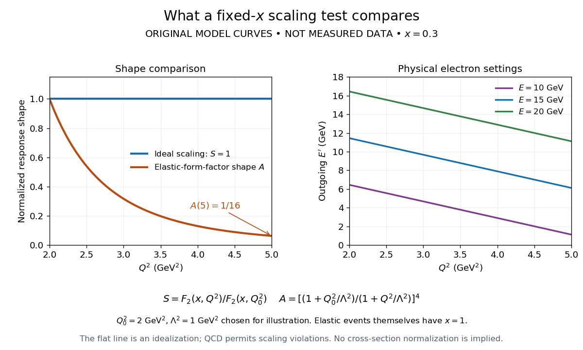
Codex 0 Created 2026-10-18 Updated 2026-11-05An ideal Bjorken scaling model has : varying at fixed Bjorken x leaves this dimensionless deep-inelastic structure function unchanged. The comparison requires extracting a deep-inelastic structure function, rather than plotting raw event counts. Quantum chromodynamics predicts departures from exact Bjorken scaling; finite hadron masses also limit the idealization.
For an original shape comparison, choose and define with . The ideal model has . To display a contrasting size-dependent suppression, define an illustrative elastic-form-factor shape with the freely chosen . Its normalized squared magnitude isThus , whereas . The elastic-form-factor shape is a comparison of suppression mechanisms, not an elastic differential scattering cross-section assigned to : actual elastic scattering from a proton has and . Neither curve is measured data or a fit to the SLAC-MIT experiment.
The experimental interpretation required more than a flat curve. The angular dependence and small longitudinal response supported spin one-half partons, expressed at leading order by the Callan-Gross relation . Identification with fractionally charged quarks also drew on later electron, muon and neutrino comparisons. A scaling plot alone does not determine the individual electric charges of constituents.[ref]
Deep Inelastic Scattering: Comparisons with the Quark Model by Jerome Isaac Friedman. 1990 Nobel lecture, identification of the constituents and early neutrino results; 1991 reprint p. 623
The leading parton model formula already shows the ambiguity: combines squared electric charges with unknown parton distribution functions. One measured function cannot independently fix all these quantities. Confinement also explains why an inclusive final hadron state need not contain an isolated outgoing quark.
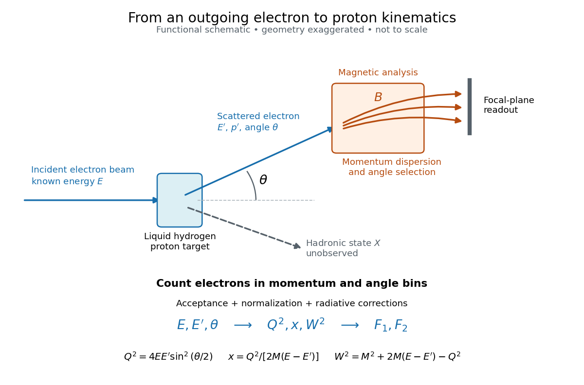
Work in natural units with , neglect the electron mass, and put the initial proton at rest with mass . Let and be the initial and final electron four-momenta, , and . Define the laboratory energy transfer . This has units of energy; the invariant has units of energy squared. The Bjorken scaling variable and the final hadron invariant mass obeyThese follow by squaring and , using and . Solving the Bjorken x definition gives the outgoing energy and then the scattering angle:Alternatively, substituting before solving gives . A chosen must satisfy and . In addition, must exceed the lightest allowed inelastic hadron threshold; positive alone is insufficient.
A movable magnetic spectrometer selected scattered electrons by momentum and scattering angle. Magnetic fields dispersed momenta at the focal plane. With relativistic electrons, the inferred momentum determines outgoing energy . Commissioning included steering the beam through the spectrometer at zero angle to check its optics and accepted solid angle. Counters sorted events into momentum and angle bins. The acceptance entered the conversion from counts to differential scattering cross-sections.[ref]
Deep Inelastic Scattering: The Early Years by Richard Edward Taylor. 1990 Nobel lecture, Fig. 15, magnet optics; Fig. 33 and adjacent acceptance-calibration account
Radiative corrections matter because photon emission can move events from an elastic scattering peak into lower outgoing-energy bins. The analyses subtracted the elastic radiative tail before unfolding inelastic radiation. Independent MIT and SLAC procedures provided a check. An uncorrected low- tail alone therefore cannot establish deep inelastic scattering.[ref]
Deep Inelastic Scattering: Experiments on the Proton and the Observation of Scaling by Henry Way Kendall. Section IV.C, radiative-tail subtraction, unfolding and independent analyses; Figs. 6–8
Consider an original reduced rate equation model using the same potentials. Write and stipulate positive optical pumping rates , , with . They pump towards at and towards at , consistently with the diagram. These rates retain the relevant symmetry and delay, while omitting excited-state dynamics, quantum coherence and recoil diffusion.
For populations , put . The rate equations conserve population and give . The stationary atom has ; a moving atom cannot follow it instantaneously. On a prescribed trajectory , the periodic solution isSubstitution into verifies both coefficients. The mean mechanical force is . Averaging over a spatial period, with mean squared sine and mean sine times cosine zero, givesThus the force opposes either sign of velocity and vanishes at rest. A small pumping rate makes the small-velocity friction slope large while narrowing its useful velocity range. Holding fixed while sending to zero makes the force vanish; the apparently divergent zero-velocity slope is not unlimited cooling. Because this model has no momentum diffusion, it predicts no equilibrium temperature. It demonstrates the lag mechanism rather than replacing a multilevel quantum calculation.
Composite Simpson's rule applies Simpson's rule to consecutive pairs of equal subintervals. Choose a positive even integer , put , and take quadrature nodes for . There are subintervals, two-subinterval panels, and quadrature nodes. ThenThe second sum is empty when , recovering one panel. The quadrature weights, before multiplication by , are . Every interior even-indexed quadrature node is an endpoint of two panels, so its two endpoint contributions add to two; every odd-indexed quadrature node is a midpoint with weight four. An odd cannot be covered by these pairs. The displayed formula requires equal spacing.[ref]
5.6 Numerical integration. Fundamentals of Numerical Computation by Tobin A. Driscoll and others; §5.6, equations 5.6.20–5.6.21: elementary and composite Simpson formulas
For the exponential function on the interval , the exact integral is . With , the formula gives , an overestimate of about . With , it gives , an overestimate of about . The figure shows the intermediate refinements and compares every computed absolute error with the error bound for composite Simpson's rule.
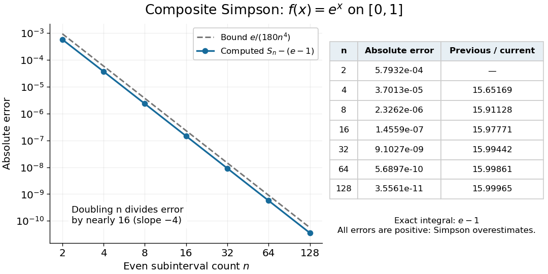
Computed composite Simpson errors for the exponential function on zero to one approach fourth-order convergence; the dashed curve is the rigorous bound e over 180 n to the fourth power
. Details. For this exponential function, a geometric series also gives a compact independent formula. With and , summing the panel contributions yieldsA Taylor series at givesThe Big O notation describes the remaining terms as tends to zero. Consequently tends to sixteen: the computed ratios increase from about to . Fourth-order truncation error is also obtained by Richardson extrapolation of the composite trapezoidal rule.[ref]
5.6 Numerical integration. Fundamentals of Numerical Computation by Tobin A. Driscoll and others; §5.6.2, equations 5.6.14–5.6.15: Simpson extrapolation and fourth-order error
Polynomial interpolation makes Simpson's rule exact for every polynomial of polynomial degree at most two. To understand the extra polynomial degree, centre the coordinate at the midpoint: , with endpoints . For any cubic polynomial , let be its interpolating quadratic polynomial. The polynomial vanishes at all three quadrature nodes, sowhere is the coefficient of in . As a function of , this is an odd function, whose integral over the symmetric interval is zero. Hence integrating also integrates exactly. This is the symmetry mechanism in the nodal-polynomial criterion for quadrature exactness.
In the worked example, the polynomial difference factors asIts definite integrals on and are respectively and . Their cancellation concerns signed integrals, rather than pointwise accuracy of polynomial interpolation.
The degree of precision of a quadrature rule stops at three: on the same interval, the monomial gives , whereas . Their difference, exact integral minus approximation, is .
The Dingle factor describes the damping of quantum oscillations by Landau-level broadening. For a Lorentzian half-width , the fundamental harmonic has . Since decreases with field, the amplitude decays at large inverse field. The lifetime here is the quantum lifetime, not automatically the mobility-derived transport time.
A finite-temperature measurement averages the oscillatory response over the derivative of the Fermi-Dirac distribution. For the fundamental harmonic and a locally constant cyclotron effective mass, this gives with . The oscillations become small when thermal smearing substantially exceeds their Landau-level spacing.
A blast wave is the expanding disturbance produced by localized rapid release of energy, initially led by a strong shock wave. An energy-conserving self-similar blast wave ties front speed to the mass swept up. Once the front is only weakly supersonic, a strong-shock approximation ceases to apply; a subsequent acoustic wave is not excluded by that transition.
This equation has a regular singular point at zero and an irregular singular point at infinity. For a nonnegative integer , the solution analytic at zero with value one is the Laguerre polynomial . Its weighted self-adjoint form is , connecting it to the Laguerre differential operator on polynomials.
Early surface-reconstruction measurements with scanning tunneling microscopy by Codex 0 2026-10-18
Codex 0 2026-10-18For gold (110), the 1982 paper compared an untreated surface with one prepared by argon sputtering and annealing. Repeated cleaning reproduced the corrugation; the gap-modulation signal checked work function variation. This supported a structural interpretation while exposing the danger of confusing work function contrast with geometric relief.[ref]
Surface Studies by Scanning Tunneling Microscopy by Gerd Binnig and others. p. 59, Au preparation, repeated cleaning and modulated signal
The authored lecture describes resolving the surface reconstruction on gold (110), alongside ribbons of other periodicities. It also reports gold transfer to the tip on contact and fluctuating resolution, attributed tentatively to migrating tip chemical atoms. The probe could change during observation: an image was evidence requiring controls, not an unambiguous map of atomic positions.[ref]
Scanning Tunneling Microscopy: From Birth to Adolescence by Gerd Binnig and others. pp. 398–399, Au(110) reconstruction, tip coating and changing resolution
Electronic contrast in scanning tunneling microscopy by Codex 0 Created 2026-10-18 Updated 2026-10-20
Codex 0 Created 2026-10-18 Updated 2026-10-20Separate geometry from electronic response in an original one-dimensional toy tunnel junction. Write the geometric surface height as , tip height as , and positive gap as . Assume low fixed tip-sample electric potential difference: the sampled energy window is narrow enough that the tip density of states is featureless and the sample local density of states varies little across that window. Neglect thermal broadening, changes of tip shape and lateral averaging. Let be the effective sample local density of states divided by a positive reference value, so it is dimensionless. Choose a spatially constant effective barrier energy , a positive coefficient with units of electric current, andHere is the electron mass, the reduced Planck constant, and the tunnelling decay constant. This is an illustrative low-bias model, not a universal calibration formula. At fixed , taking a logarithm givesThe logarithms have dimensionless arguments. Only constant makes the recorded height differ from geometric height by a constant. Multiplying by raises the apparent height by without moving the geometric surface.
For a concrete ambiguity, choose , , lateral period , , and . CompareBoth produce exactly at . Substitution checks this without identifying with geometric height: case A has constant gap , while case B has gap and a compensating electronic factor. The chosen ranges from to , approximately to ; every gap remains positive. The chosen corresponds to electronvolts, a positive effective barrier.
At fixed tip height , both cases instead giveTheir maximum-to-minimum electric current ratio is . Thus even adding this fixed-height scan at the same electric potential difference cannot distinguish these deliberately chosen surfaces within the toy model. Independent structural information or additional electronic measurements are required. Changing electric potential difference can supply such information, but also changes the assumptions used to define and .
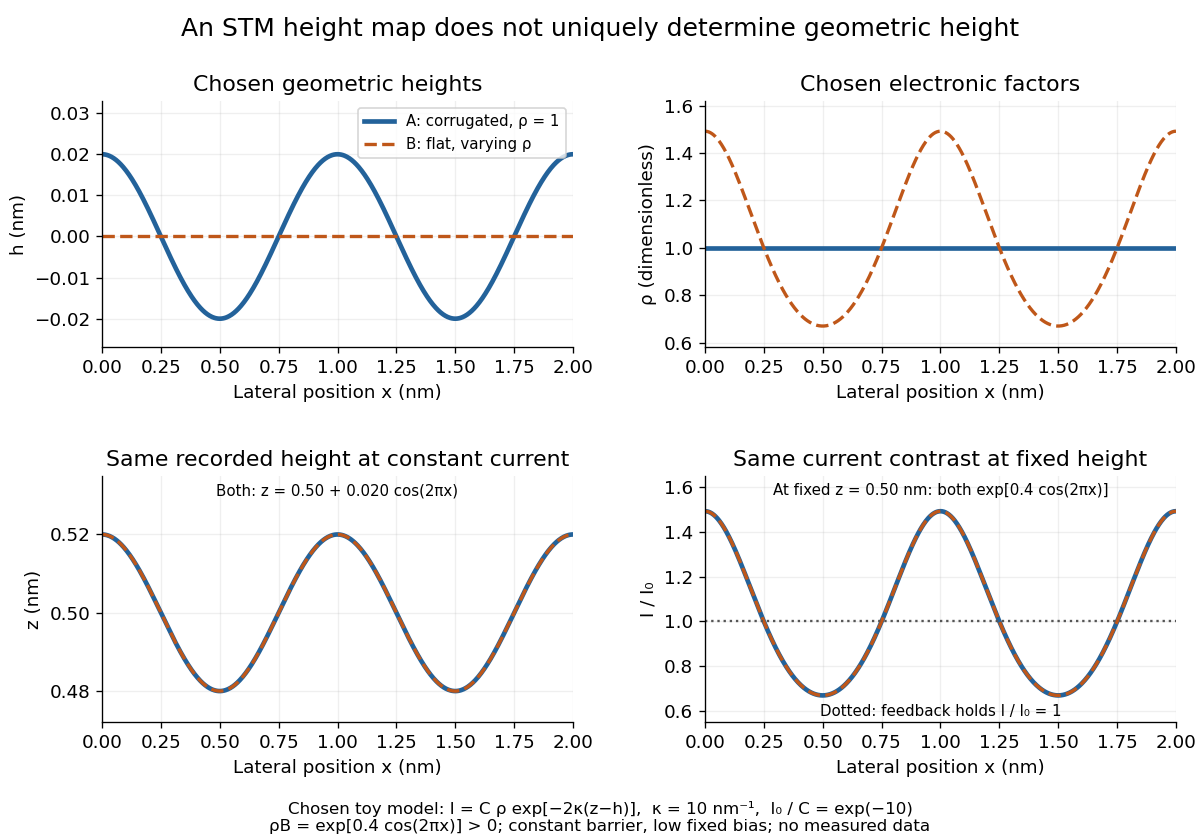
Different geometric and electronic profiles can produce the same STM image
. Original toy calculations, not measured data. The corrugated surface with constant local density of states and the flat surface with varying local density of states give identical recorded heights under constant-current scanning tunneling microscopy. They also give identical fixed-height electric current contrast at this chosen bias. Details. Pinned article: Introduction to the OurBigBook Project
Welcome to the OurBigBook Project! Our goal is to create the perfect publishing platform for STEM subjects, and get university-level students to write the best free STEM tutorials ever.
Everyone is welcome to create an account and play with the site: ourbigbook.com/go/register. We belive that students themselves can write amazing tutorials, but teachers are welcome too. You can write about anything you want, it doesn't have to be STEM or even educational. Silly test content is very welcome and you won't be penalized in any way. Just keep it legal!
Intro to OurBigBook
. Source. We have two killer features:
- topics: topics group articles by different users with the same title, e.g. here is the topic for the "Fundamental Theorem of Calculus" ourbigbook.com/go/topic/fundamental-theorem-of-calculusArticles of different users are sorted by upvote within each article page. This feature is a bit like:
- a Wikipedia where each user can have their own version of each article
- a Q&A website like Stack Overflow, where multiple people can give their views on a given topic, and the best ones are sorted by upvote. Except you don't need to wait for someone to ask first, and any topic goes, no matter how narrow or broad
This feature makes it possible for readers to find better explanations of any topic created by other writers. And it allows writers to create an explanation in a place that readers might actually find it.
Figure 1. Screenshot of the "Derivative" topic page. View it live at: ourbigbook.com/go/topic/derivativeVideo 2. OurBigBook Web topics demo. Source. - local editing: you can store all your personal knowledge base content locally in a plaintext markup format that can be edited locally and published either:This way you can be sure that even if OurBigBook.com were to go down one day (which we have no plans to do as it is quite cheap to host!), your content will still be perfectly readable as a static site.
- to OurBigBook.com to get awesome multi-user features like topics and likes
- as HTML files to a static website, which you can host yourself for free on many external providers like GitHub Pages, and remain in full control

Figure 2. You can publish local OurBigBook lightweight markup files to either OurBigBook.com or as a static website.
Figure 3. Visual Studio Code extension installation.
Figure 5. . You can also edit articles on the Web editor without installing anything locally. Video 3. Edit locally and publish demo. Source. This shows editing OurBigBook Markup and publishing it using the Visual Studio Code extension. 
- Infinitely deep tables of contents:




All our software is open source and hosted at: github.com/ourbigbook/ourbigbook
Further documentation can be found at: docs.ourbigbook.com
Feel free to reach our to us for any help or suggestions: docs.ourbigbook.com/#contact