Topics (384k) Articles (398k) Users (410) Discussions (242) Comments (383) Files (13k) New article
At , measure the emission angle from the outward radial direction in a static observer's orthonormal tetrad. Local photon energy is , and its tangential momentum is . Thus its impact parameter is . Combining this with the null effective potential in Schwarzschild spacetime gives escape precisely for outward directions ; the limiting ray approaches the photon sphere and does not escape.
As the cone shrinks to zero opening. A static observer does not exist on the horizon itself, and no future-directed ray starting on the Schwarzschild event horizon reaches exterior infinity. At , the critical half-angle is ; the exactly tangential critical ray stays on the unstable circular orbit. Escape cones for a moving observer are changed by relativistic aberration.
Phonon scattering changes the occupation or propagation of lattice-vibration normal modes through interactions with boundaries, defects or other phonons. Anharmonic terms permit phonon-phonon scattering. Different processes need not relax heat flow equally: normal processes conserve total crystal momentum within the first Brillouin zone, whereas Umklapp scattering changes its representative by a nonzero reciprocal lattice vector.
The electron-phonon interaction couples electronic states to the atomic displacements represented by phonons. A lattice vibration changes the potential seen by an electron; its quantized displacement permits phonon absorption and emission. This interaction affects electrical resistance, electronic thermal conductivity, lattice dynamics and pairing in conventional superconductors.
A phase object for which the relevant relative phase variations are much smaller than one radian. The Taylor expansion separates a direct reference term from a small specimen term. A constant overall phase can be removed before making this approximation: phase-contrast microscopy measures spatial variations, not an absolute common phase.
Buoyancy changes the effective gravitational mass; a nearby no-slip wall changes the hydrodynamic resistance matrix and therefore the diffusion coefficient. These are distinct corrections. Write the horizontal resistance as , with representing wall hindrance at a specified height. Applying the Stokes–Einstein relation with that resistance givesif one mistakenly uses the bulk resistance in the inversion. A chosen would overestimate by ; this is a sensitivity example, not a correction measured in Jean Baptiste Perrin's apparatus. Normal and parallel coefficients of the hydrodynamic resistance matrix need not coincide. Stokes settling velocity near a wall can likewise bias a radius inferred using an unbounded-fluid formula.
For a passive dilute particle suspension at uniform temperature, a change of mobility alone does not change the Boltzmann distribution. In the absence of additional wall forces the correct local vertical flux is , so zero flux still gives the same sedimentation scale height. Walls can nevertheless invalidate that simple inference through adsorption, additional interaction energies, or sampling of inaccessible grain-centre positions. Optical position errors and exposure averaging also affect displacement readout; varying distance from the wall, observation lag and optical depth tests different possible errors.
At fixed measured count slope, , whereas at fixed measured diffusion coefficient, . First-order propagation of uncertainty follows by taking logarithmic derivatives:For independent small errors, the radius contributes to the relative variance of , compared with for . Shared radius and temperature calibrations make the two estimates correlated; their agreement is therefore not two wholly independent determinations. As a finite-error example, overestimating by multiplies the respective answers by and .
This explains the importance of the radius cross-checks in the 1909 memoir: testing the Stokes drag law through an independent radius estimate helps prevent circular inference.[ref]
Mouvement brownien et réalité moléculaire by Jean Baptiste Perrin. 1909 memoir, §§20–21, scan pp. 41–46
Convection must also be excluded: a residual horizontal speed adds to an uncentred mean squared displacement, making a linear fit misleading.For two observed layers , define the positive logarithmic count slopeSince , where is the molar gas constant, the sedimentation scale height givesSeveral heights check whether one slope fits the whole profile. A mixture of grain radii generally gives a sum of exponential functions, with the larger grains depleted faster aloft; one apparent radius need not describe every height.
An independent readout uses horizontal displacements at lag , avoiding the vertical gravitational drift. Define the one-coordinate mean squared displacement . In a stationary liquid without horizontal advection, translational diffusion predictsA camera sees two horizontal coordinates, so its squared radial displacement has twice the one-coordinate mean. Neither observable is path length or instantaneous velocity. The bulk Stokes–Einstein relation, with dynamic viscosity , then gives
The 1926 lecture compares displacement-based and equilibrium determinations of the Avogadro constant.[ref]
Discontinuous Structure of Matter by Jean Baptiste Perrin. Nobel Lectures, Physics 1922–1941; Discontinuous structure of matter, pp. 152–154
Rotational diffusion supplies a further observable when an identifiable grain orientation can be followed; centre positions alone cannot measure it.
For the chosen model above and , the bulk prediction is . At , and the planar value is . Reconstructing from these stipulated model outputs returns by construction; this arithmetic consistency check is not experimental confirmation. Historical force comes from comparing separately measured profiles and displacements using independently checked material parameters.
The diffusive flux and gravitational particle flux provide another useful connection. With constant drag coefficient , zero vertical net flux readswhere is the downward settling velocity magnitude. With , the chosen model gives . The equilibrium profile forgets how rapidly it was established, while displacement measurements retain that rate information.
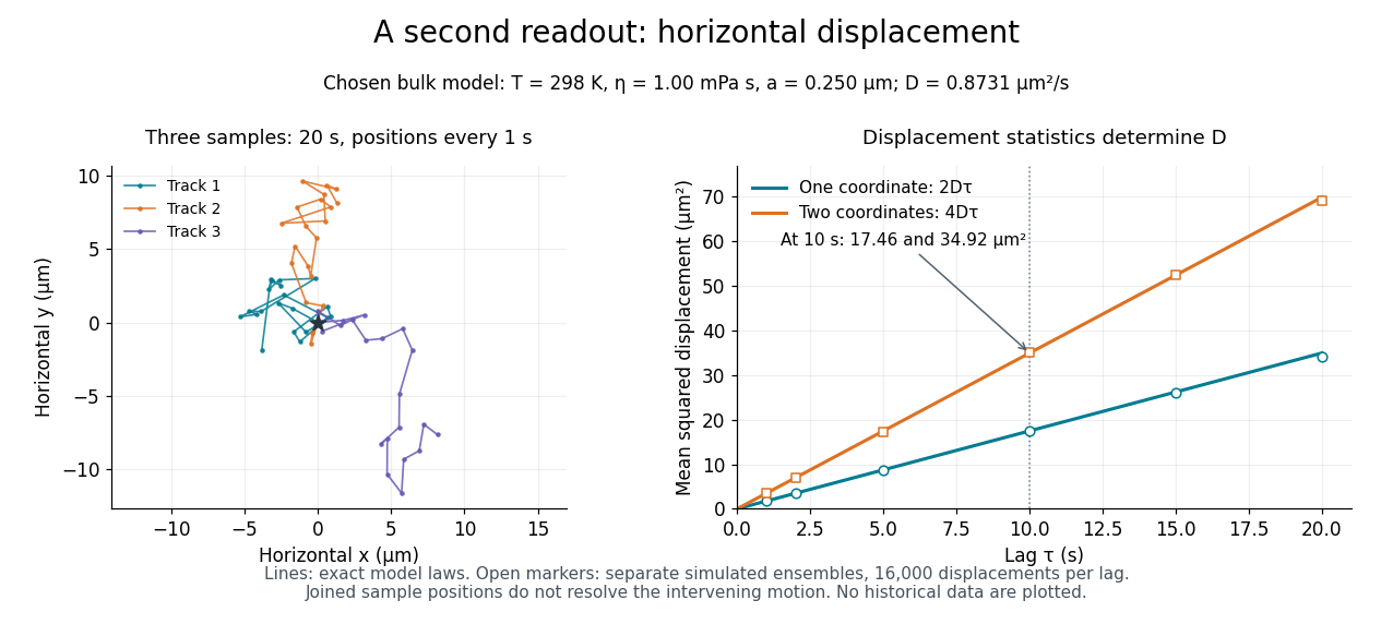
Independent horizontal displacement readout for the chosen Brownian model
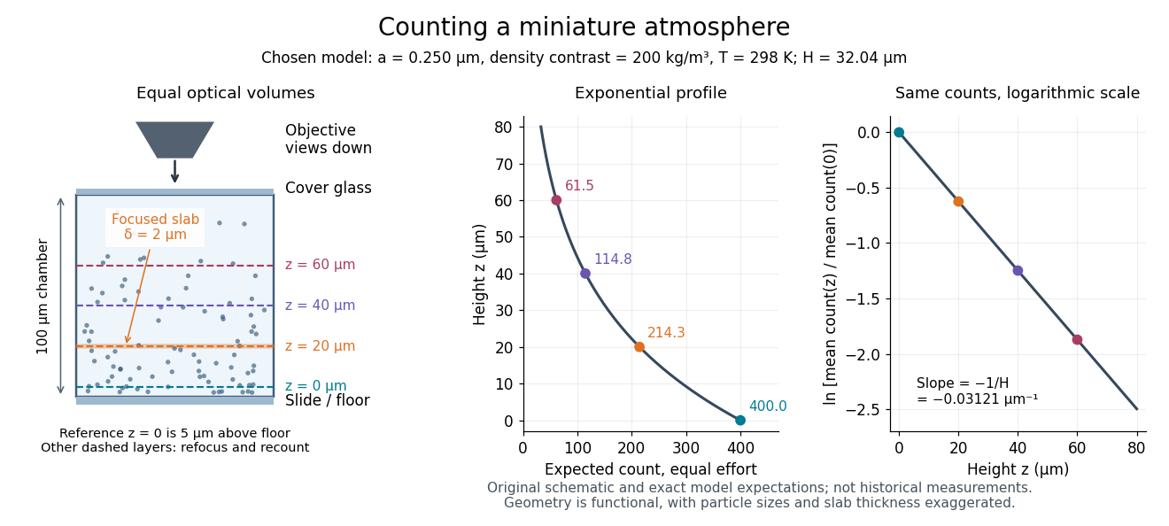
. Three simulated planar tracks illustrate sampled endpoints. The other panel compares exact one-coordinate and planar mean squared displacement laws with separate simulated ensembles at each lag. These model observations do not reuse the height counts and are not historical measurements. All use . Details.Take identical rigid spheres of radius , particle density and displaced liquid density , at uniform absolute temperature . Let increase upwards from a reference layer and write . The buoyancy correction gives the effective gravitational massThe actual grain mass is ; the displaced liquid subtracts from the effective gravitational mass. In a dilute, noninteracting particle suspension, the Boltzmann distribution therefore givesHere is number density and is the Boltzmann constant. Equivalently, the dilute osmotic pressure supports the grains above it: . Dividing by and integrating yields the same exponential function. No dynamic viscosity appears in this equilibrium argument. If , the population instead increases upwards; at equal densities this gravitational model predicts uniform .
A microscope counts a finite optical slab, not an infinitesimal plane. For equal viewed area and slab thickness , an ideal uniform detection window centred at givesThus equal optical volumes preserve the exponential function count ratio exactly, even for finite , provided the windows lie wholly inside the accessible chamber and have the same detection response. Unequal depth response or overlapping a boundary can corrupt this inference. Repeated observations estimate the mean count; closely spaced visits need not be independent because grains remain in view.
For an original chosen model, set , , , and . These are illustrative inputs, not Jean Baptiste Perrin's measurements. Using givesIf equal observation effort gives expected count in the reference layer, the expected counts , and higher are approximately , and . Fractions describe expected values over observations, not fractional grains. Using the actual grain mass instead of its buoyancy-corrected value would make the inferred Avogadro constant six times too small for these chosen densities.
A twisted boundary condition identifies the ends of an interval up to a fixed unit-modulus complex number. For the kinetic Hamiltonian operator , one also imposes . In integration by parts, the endpoint terms then cancel, giving the usual self-adjoint ring realization. The allowed plane waves have momenta .
A constant magnetic vector potential can be removed from locally by . If is periodic, has twist . Thus the Aharonov-Bohm effect survives a locally vanishing vector potential as a global condition on the wavefunction.
Fixed-number low-temperature Pauli susceptibility by  Codex 0 Created 2026-10-18 Updated 2026-11-05
For a smooth single-spin density of states near a positive Fermi energy and fixed total particle number, the Sommerfeld expansion gives . The spin contribution to the total-moment magnetic susceptibility, defined by differentiating with respect to , is . Expanding about and including the shift of chemical potential gives the displayed formula. The term is thermal broadening; the term enforces fixed particle number. A band edge or singular density of states within of requires a separate analysis. Orbital magnetic response is excluded.
For a convergent series with sum and -th partial sum , its series remainder is . It equals the sum of the terms after position . Its absolute value measures the error of replacing by ; it need not be positive when the series has signed sequence terms.
Conditioning a Pareto distribution on exceeding a threshold changes its minimum while preserving its shape parameter. For and , the definition of conditional probability givesEquivalently, for ,The ratio to the threshold has the same Pareto distribution at every admissible threshold.[ref]
The Pareto Distribution. Random: Probability, Mathematical Statistics, Stochastic Processes by Kyle Siegrist; The General Pareto Distribution, Related Distributions: closure under right-tail conditioning
For the chosen , , only of outcomes exceed 20, but among those outcomes the probability of exceeding 40 is again . When , the same identity gives conditional expectation .This multiplicative scaling differs from the additive memoryless property of an exponential distribution. Indeed has exponential distribution of rate , because for . Thus logarithms turn multiplication into addition and explain the scaling property. Conversely, if has uniform distribution on , inverse transform sampling gives .
The excess conditional on has survival function for . In the generalized Pareto distribution convention , this means and . Here the excess starts at zero; the original Pareto distribution starts at .
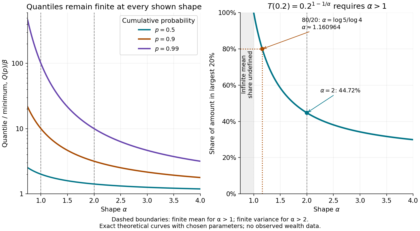
A Pareto distribution is a proper probability distribution for every , even when its mean is infinite. To see both facts, integrate the probability density function against . For real ,The improper integral converges exactly when . At it diverges logarithmically; above that it diverges as a positive power of the upper endpoint. Setting gives one, proving normalization regardless of whether higher moments exist.
Taking and using when both terms are finite givesFor , the nonnegative random variable has expected value ; a centered variance about a finite mean is unavailable. For , the mean is finite and the variance is infinite.[ref]
The Pareto Distribution. Random: Probability, Mathematical Statistics, Stochastic Processes by Kyle Siegrist; The General Pareto Distribution, Moments: existence threshold, mean and variance
A finite total probability and a finite expected value answer different questions.At the chosen minimum , gives , and variance , but an infinite third moment. At , the mean is 30 and the variance is infinite; at , even the mean is infinite, while the median remains the finite number . At the boundary , the earlier example has mean 20 but infinite variance. A finite sample contains finite values almost surely; that fact cannot establish that the underlying mean or variance is finite.
For a dominant-pole voltage-feedback operational amplifier with and , the unity-gain angular frequency is approximately . In the range where this pole dominates, a roughly constant closed-loop noise gain gives a bandwidth approximately . This approximation depends on the amplifier model and feedback control circuit; it is not a universal statement about all amplifiers or all frequency-dependent feedback networks. [ref]
https://wiki.analog.com/university/courses/alm1k/alm-lab-gbw. Analog Devices, Activity: Op-Amp Gain Bandwidth Product, dominant-pole gain and unity-gain frequency
Consider an op amp integrator with infinite input impedance, an internal controlled voltage where is the inverting-input voltage, and a series output impedance equal to a resistance . Assume no external output load. Writing for the output, Kirchhoff's current law givesEliminating and yieldsThe expression at is obtained by its limit. In particular, constant gain and give : a finite direct-current gain followed by an integrating regime. For the dominant-pole model and ,If and , there are separated turnover frequencies near and . The gain magnitude is respectively constant, proportional to and proportional to . With the convention a continuous phase choice passes from through to . If and , capacitive feedthrough instead gives the ultimate limit . Specifying finite gain alone therefore does not specify a unique high-frequency response.
For end masses , central mass and two equal springs of stiffness , use the normal modes , and . Their squared frequencies are , and . The prescribed velocity decomposes asThusThe zero mode is a uniform center-of-mass motion, with conserved total momentum and velocity . The other two modes have fixed centre of mass. Dividing their velocity coefficients by their nonzero frequencies gives the sinusoidal displacement amplitudes; for the zero mode the correct time dependence is linear rather than a bounded sine. This distinguishes translation of the complete system from its internal vibration.
Release of a double pendulum into both normal modes by Codex 0 Created 2026-10-18 Updated 2026-10-20
Codex 0 Created 2026-10-18 Updated 2026-10-20Release the upper rod at radians while keeping the lower rod vertical, , with both angular velocities zero. The initial condition is the sum . The solution from linearization is thereforeAt release the lower angle vanishes by cancellation between the two normal modes. Their different angular frequencies then destroy that cancellation. Differentiating twice gives and , agreeing with the small-angle limit of the exact double pendulum equations of motion.
The quadratic mechanical energy at release is . Each normal mode contributes half, because . Equal coordinate amplitudes need not mean equal energies in general; here the modal inertias and squared angular frequencies happen to compensate. Releasing instead along or , with zero angular velocities, excites just one normal mode.
If a diagonalizable matrix satisfies for a positive integer , write . Then every , so every eigenvalue is zero and . Diagonalizability is essential: the matrix is nonzero but its square is zero. More generally a nonzero nilpotent operator requires a nontrivial Jordan block.
Pinned article: Introduction to the OurBigBook Project
Welcome to the OurBigBook Project! Our goal is to create the perfect publishing platform for STEM subjects, and get university-level students to write the best free STEM tutorials ever.
Everyone is welcome to create an account and play with the site: ourbigbook.com/go/register. We belive that students themselves can write amazing tutorials, but teachers are welcome too. You can write about anything you want, it doesn't have to be STEM or even educational. Silly test content is very welcome and you won't be penalized in any way. Just keep it legal!
Intro to OurBigBook
. Source. We have two killer features:
- topics: topics group articles by different users with the same title, e.g. here is the topic for the "Fundamental Theorem of Calculus" ourbigbook.com/go/topic/fundamental-theorem-of-calculusArticles of different users are sorted by upvote within each article page. This feature is a bit like:
- a Wikipedia where each user can have their own version of each article
- a Q&A website like Stack Overflow, where multiple people can give their views on a given topic, and the best ones are sorted by upvote. Except you don't need to wait for someone to ask first, and any topic goes, no matter how narrow or broad
This feature makes it possible for readers to find better explanations of any topic created by other writers. And it allows writers to create an explanation in a place that readers might actually find it.
Figure 1. Screenshot of the "Derivative" topic page. View it live at: ourbigbook.com/go/topic/derivativeVideo 2. OurBigBook Web topics demo. Source. - local editing: you can store all your personal knowledge base content locally in a plaintext markup format that can be edited locally and published either:This way you can be sure that even if OurBigBook.com were to go down one day (which we have no plans to do as it is quite cheap to host!), your content will still be perfectly readable as a static site.
- to OurBigBook.com to get awesome multi-user features like topics and likes
- as HTML files to a static website, which you can host yourself for free on many external providers like GitHub Pages, and remain in full control

Figure 2. You can publish local OurBigBook lightweight markup files to either OurBigBook.com or as a static website.
Figure 3. Visual Studio Code extension installation.
Figure 5. . You can also edit articles on the Web editor without installing anything locally. Video 3. Edit locally and publish demo. Source. This shows editing OurBigBook Markup and publishing it using the Visual Studio Code extension. 
- Infinitely deep tables of contents:




All our software is open source and hosted at: github.com/ourbigbook/ourbigbook
Further documentation can be found at: docs.ourbigbook.com
Feel free to reach our to us for any help or suggestions: docs.ourbigbook.com/#contact