Topics (384k) Articles (398k) Users (410) Discussions (242) Comments (383) Files (13k) New article
Choose a fixed tip-sample electric potential difference and a positive target electric current magnitude . At each lateral position , feedback control adjusts until the measured electric current approaches . Since increasing the gap reduces quantum tunnelling, excessive electric current calls for retraction; insufficient electric current calls for approach. The image is the calibrated vertical displacement , while the residual electric current error tests how closely the loop followed its target.
This is a contour of equal electric current, not necessarily a contour of equal separation. The electronic contrast in scanning tunneling microscopy model below shows why. It also explains the value of vibration isolation: an unintended displacement changes the same sensitive gap as the feature being measured. A scan must be slow enough for the finite bandwidth of feedback control; otherwise lags the desired contour.
Work over the rational numbers, allowing unknowns in the real numbers when interpreting the geometry. Consider four equations in three unknowns:The third row of is the sum of its first two rows, and the fourth is their difference, second minus first. The same relations must hold on the right: consistency requires and . The latter condition already holds. Gaussian elimination makes this compatibility test explicit while exposing the remaining freedom.
Apply the elementary row operations in this order, using each row's current value:then and . The resulting augmented matrix is in row echelon form for every :When , the third row has its pivot element in the augmented column. It says , so the linear system has no solution. When , that entire row vanishes and only two pivot elements remain. More equations than unknowns therefore do not force a unique solution: some equations may repeat information.
The final operation reduces the coefficient block toThe product of all six elementary matrices isDirect matrix multiplication verifies both displayed transformations. Its determinant is one, so this transformation is reversible. In particular, the third row of extracts the discrepancy between the third equation and the sum of the first two.
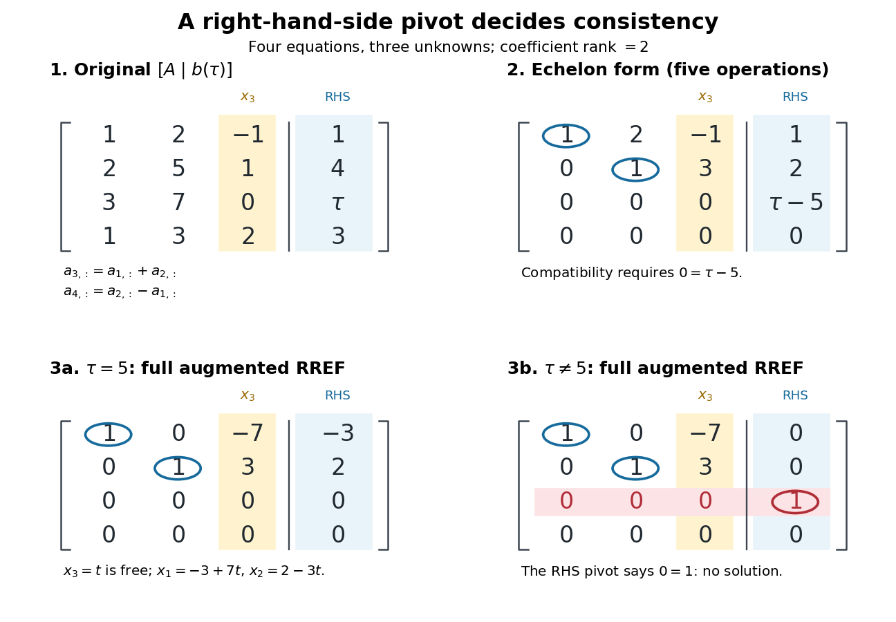
Row echelon form exposes compatibility; a right-hand-side pivot element distinguishes inconsistency from a free variable in a linear system
. Details. For , is the reduced row echelon form of the full augmented matrix. For , only its coefficient block is reduced: scale the third row by and clear the entries above its augmented pivot element. The full reduced row echelon form is thenThe last column is part of the matrix when testing the echelon conditions. Calling fully reduced before clearing that column would miss this distinction.
Two matrices of the same size over the same field are row-equivalent matrices if a sequence of elementary row operations transforms one into the other.[ref]
Row Reduction. Interactive Linear Algebra by Dan Margalit and others; §1.2.1, definition of row equivalence
Every operation is reversible, so they have the same row space and the same column linear relations. Writing the entire sequence as multiplication by an invertible matrix gives andThus the kernel is preserved. For a nonzero right-hand side, perform every operation on the whole augmented matrix : changing the coefficients while keeping fixed generally changes the solutions. The column space instead transforms to , which need not equal .Let and for the conditional distributions of parahydrogen and orthohydrogen, with . Differentiating the normalized Boltzmann factors gives . Thus the rotational heat capacity at constant volume per molecule of a composition frozen at isAt conversion equilibrium, the law of total variance adds a nonnegative contribution from the changing species populations:The last term is the contribution from conversion. Compare the first two terms with a frozen sample at the same instantaneous composition; a frozen sample generally has different weights too. This formula follows directly from the variance of a mixture: subtract the overall mean inside each species, expand the square, and the cross terms vanish because each conditional deviation has zero mean. It also proves nonnegative rotational heat capacity in either model.
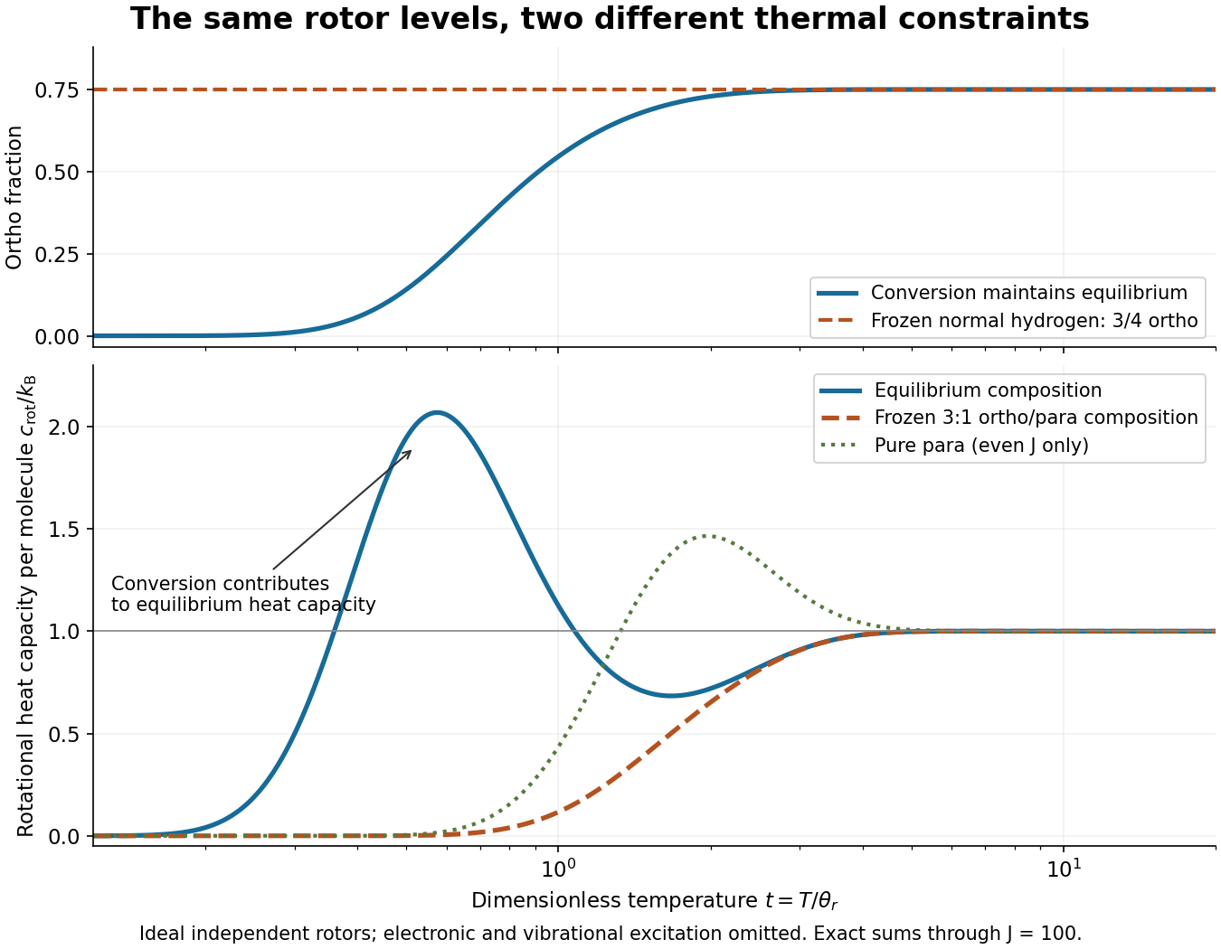
For an original worked example at , summing the allowed ladders gives , , and . The calculated rotational heat capacities are and for frozen normal hydrogen. The contrast is large because changing species accesses the to separation, whereas fixed species must use the larger to or to separations. These are model numbers at a chosen dimensionless temperature, not measured hydrogen data.
Both rotational heat capacities approach zero as , although frozen normal hydrogen retains nonzero rotational internal energy. Both approach as within the rotor model. The high-temperature limit is a formal limit with all other excitations suppressed; actual molecular hydrogen eventually needs molecular vibration, nonrigidity, and dissociation. Multiplying the per-molecule result by the Avogadro constant gives rotational molar heat capacity in units of the molar gas constant . A dilute classical ideal gas additionally contributes from translation to its heat capacity at constant volume.
A solid torus of major radius and minor radius , centred on the horizontal plane, has volume . In circular torus coordinates, . Integrating with the Jacobian determinant gives ; the part odd in vanishes. Thus the mean squared height is . The identity is useful for moments of inertia and flux calculations using the divergence theorem.
For scalar electrical conductivity and constant permeability , the moving-fluid Ohm law and the quasistatic Ampere-Maxwell law give , where is the magnetic diffusivity. Taking minus the curl and using Faraday's law of induction gives . Expanding this expression and imposing yields the title equation. The familiar constant-diffusivity resistive induction equation omits the last term because ; nonrelativistic motion alone does not establish that simplification.
A thermistor is a temperature-sensitive resistor used as a resistance thermometer. Its calibrated electrical resistance supplies a temperature indication; probe heat capacity and unwanted thermal conduction can affect its response and immersion error.
Under the convention , choose with constant and null . The trace-reversed metric perturbation has amplitudeIt satisfies and , so it is an allowed residual gauge symmetry of linearized gravity. Its linearized Riemann curvature operator is zero: the four wavevector factors in each second-derivative term cancel in the antisymmetric curvature combinations. Nonzero transverse-traceless curvature distinguishes the two physical gravitational wave polarizations from these coordinate modes.[ref]
https://www.damtp.cam.ac.uk/user/tong/gr/grhtml/S5.html. Section 5.3.1, equations 5.232–5.234: residual plane-wave gauge transformation and transverse-traceless reduction
A technical replicate repeats a measurement or analytical procedure on the same biological preparation. For example, read the length of the same leaf three times to assess measurement error. Measuring three different leaves within one pot instead samples variation within the plant; it should be described explicitly rather than silently equated with repeated readings of one leaf. Neither procedure supplies another pot-level treatment replicate.
A biological replicate repeats a procedure using a distinct biological preparation, such as another plant or a separately established cell culture. The relevant level must be specified: several cell cultures derived from one donor can still form nested measurements for a donor-level question. Calling a sample a biological replicate does not by itself establish an independent experimental unit.
Nested measurements are responses grouped inside larger units, with each measured object belonging to just one such unit. Three leaves within each pot give nested measurements; repeatedly reading one leaf gives another level of repetition. Either can yield clustered data. A common random effect can describe the shared influence of the containing experimental unit.
For the constructed pot example, label treatments by , pots within each group by , and leaves within each pot by . Consider the statistical modelHere is a leaf length, is its group expected value, is a pot random effect, and describes remaining variation among leaves and measurement error. Assume that all pot random effects are mutually independent, all remaining errors are mutually independent, and the two collections are independent of one another and of the randomization. These are explicit modelling assumptions, conditional on the assigned treatments; no normal distribution assumption is needed for the following variance calculation.
Two distinct leaf measurements in one pot share . Their covariance is , their individual variance is , and their intraclass correlation coefficient isMeasurements from different pots have zero covariance and are independent under the stated statistical model. Statistical independence therefore concerns the whole response structure, not just the fact that the measured leaves are different objects.
Four-point regular representation of the Klein four-group by  Codex 0 Created 2026-10-18 Updated 2026-10-25
The permutation matrices of the three displayed double transpositions, together with , form a faithful representation of the Klein four-group. They satisfy and . Every nonidentity element fixes no basis vector, so this is its four-dimensional regular representation.
The constant vector spans a nonzero proper invariant subspace, proving reducibility. More completely, the columns ofform a common orthonormal basis of eigenvectors. Direct multiplication gives and . Thus the representation splits into the four distinct real one-dimensional characters, each once. The basis change is a normalized Hadamard matrix.
A frameshift mutation changes downstream grouping into codons through insertion or deletion of a number of nucleotides not divisible by three. In the constructed messenger RNA example, insert C immediately after AUG while retaining the same initiation position: . The first codon is preserved, but the original downstream groups GCU, UUC and UGA disappear. The displayed fragment now has no complete standard stop codon; what happens later depends on its continuation.
The short proof is positional: every downstream nucleotide moves by positions after an insertion of length . Boundaries recur every three positions, so they retain the original phase exactly when is divisible by three. An insertion of three nucleotides can still change the peptide, but it does not shift the downstream reading frame. This distinction helps interpret genetic variants without predicting a particular phenotype from grouping alone.[ref]
Biology 2e by Mary Ann Clark and others. §15.1, The Genetic Code, Figure 15.5: nucleotide deletion and shifted grouping
For in a sphere of radius , with zero surface density and regularity at the origin, the lowest spherically symmetric normal mode is . Substitution of in the radial Laplacian gives , and regularity removes the cosine solution. The Dirichlet boundary condition gives ; a radial mode with no interior zeros requires . Thus diffusion leakage suppresses growth below the displayed threshold, while the mode is stationary at equality. The expression at uses its continuous limit. In a linear neutron multiplication model this is the competition between bulk production and surface loss.
Compact cosine trial bound for the quantum harmonic oscillator by Codex 0 Created 2026-10-18 Updated 2026-11-05
Codex 0 Created 2026-10-18 Updated 2026-11-05For the dimensionless quantum harmonic oscillator , use the compactly supported trial on and zero elsewhere, with . It is continuous and belongs to the oscillator energy quadratic form domain: its weak derivative is square-integrable even though its ordinary derivative jumps at the endpoints. Exact integration givesThe minimum occurs at , giving the displayed upper bound, approximately , compared with exact ground state value . This illustrates why Rayleigh-Ritz variational principle trials need the energy form domain rather than the smaller operator domain.
Two-sine variational bound for a Dirichlet Mathieu equation by Codex 0 Created 2026-10-18 Updated 2026-11-05
Codex 0 Created 2026-10-18 Updated 2026-11-05For on with zero Dirichlet boundary conditions, use . Its Rayleigh quotient is . In the normalized sine basis the restricted operator has matrix . Its smaller eigenvalue gives the displayed upper bound, attained within this trial space at . The other stationary parameter gives the larger restricted eigenvalue. This is a finite-dimensional Rayleigh-Ritz method for a regular Sturm-Liouville problem with a sign-changing potential.
For axisymmetric heat conduction in a unit disk, separated modes satisfy , with weight , outer Dirichlet boundary condition , and zero radial flux at the origin. Integration by parts gives the displayed Rayleigh quotient. Its Euler-Lagrange equation under fixed recovers the mode equation; the natural endpoint term is . The Rayleigh-Ritz variational principle says that every admissible nonzero trial profile gives an upper bound on the bottom of the spectrum, and on the lowest eigenvalue when this bottom is attained by a fundamental diffusion mode. Finite weighted energy, rather than pointwise existence of a second derivative at the origin, is the relevant trial admissibility requirement.
Choose a nonzero smooth bounded profile supported in , constant near zero, and set . Its radial diffusion Rayleigh quotient isFor this tends to zero, proving that there is no positive spectral gap. Zero is not an eigenvalue with the outer Dirichlet boundary condition: zero energy would force on , hence . Thus the bottom is not attained, and a lowest exponentially decaying fundamental diffusion mode must not be assumed merely because the spatial region is bounded.
For the Dirichlet boundary conditions on , take the two-dimensional even trial space spanned by and . Using the kinetic-energy quadratic form gives, for ,The minimum occurs at and equals . It is slightly above the exact infinite square well coefficient . The zero extension of a trial function has derivative jumps at the walls, so the appropriate admissibility statement uses the Dirichlet kinetic-energy form; it need not belong to the unrestricted full-line second-derivative operator domain.
Pinned article: Introduction to the OurBigBook Project
Welcome to the OurBigBook Project! Our goal is to create the perfect publishing platform for STEM subjects, and get university-level students to write the best free STEM tutorials ever.
Everyone is welcome to create an account and play with the site: ourbigbook.com/go/register. We belive that students themselves can write amazing tutorials, but teachers are welcome too. You can write about anything you want, it doesn't have to be STEM or even educational. Silly test content is very welcome and you won't be penalized in any way. Just keep it legal!
Intro to OurBigBook
. Source. We have two killer features:
- topics: topics group articles by different users with the same title, e.g. here is the topic for the "Fundamental Theorem of Calculus" ourbigbook.com/go/topic/fundamental-theorem-of-calculusArticles of different users are sorted by upvote within each article page. This feature is a bit like:
- a Wikipedia where each user can have their own version of each article
- a Q&A website like Stack Overflow, where multiple people can give their views on a given topic, and the best ones are sorted by upvote. Except you don't need to wait for someone to ask first, and any topic goes, no matter how narrow or broad
This feature makes it possible for readers to find better explanations of any topic created by other writers. And it allows writers to create an explanation in a place that readers might actually find it.
Figure 1. Screenshot of the "Derivative" topic page. View it live at: ourbigbook.com/go/topic/derivativeVideo 2. OurBigBook Web topics demo. Source. - local editing: you can store all your personal knowledge base content locally in a plaintext markup format that can be edited locally and published either:This way you can be sure that even if OurBigBook.com were to go down one day (which we have no plans to do as it is quite cheap to host!), your content will still be perfectly readable as a static site.
- to OurBigBook.com to get awesome multi-user features like topics and likes
- as HTML files to a static website, which you can host yourself for free on many external providers like GitHub Pages, and remain in full control

Figure 2. You can publish local OurBigBook lightweight markup files to either OurBigBook.com or as a static website.
Figure 3. Visual Studio Code extension installation.
Figure 5. . You can also edit articles on the Web editor without installing anything locally. Video 3. Edit locally and publish demo. Source. This shows editing OurBigBook Markup and publishing it using the Visual Studio Code extension. 
- Infinitely deep tables of contents:




All our software is open source and hosted at: github.com/ourbigbook/ourbigbook
Further documentation can be found at: docs.ourbigbook.com
Feel free to reach our to us for any help or suggestions: docs.ourbigbook.com/#contact