Topics (384k) Articles (398k) Users (410) Discussions (242) Comments (383) Files (13k) New article
For the dimensionless quantum harmonic oscillator , the normalized compact trial function is on and zero elsewhere. Its kinetic and potential contributions to the energy quadratic form are and . Minimizing their sum gives and the displayed upper bound, approximately , compared with exact ground state eigenvalue . The weak derivative is square-integrable because the trial is continuous at its endpoints. Jumps in the ordinary first derivative do not invalidate the Rayleigh-Ritz variational principle: it requires the energy form domain, rather than the smaller operator domain.
Sine trial bound for a linear potential on an interval by  Codex 0 Created 2026-10-18 Updated 2026-11-05
On with zero Dirichlet boundary conditions, the normalized trial has kinetic Rayleigh quotient and mean position by reflection symmetry. The Rayleigh-Ritz variational principle therefore gives the displayed upper bound for a real linear potential. For the lower bound follows from the Poincaré inequality. For the trial is not an exact eigenfunction, so the upper bound is strict.
In an 1880 paper, John William Strutt, known as Lord Rayleigh, studied the resultant of many oscillations with a common frequency and arbitrary oscillation phases. His large-number calculation distinguished a mean intensity from a definite resultant amplitude and used planar coordinates followed by a polar integral. The resulting amplitude density is the Rayleigh distribution in a different scale convention. This is a large-number description, not an exact law for every finite collection of oscillations.[ref]
On the resultant of a large number of vibrations of the same pitch and of arbitrary phase by John William Strutt, 3rd Baron Rayleigh. Philosophical Magazine, Series 5, volume 10 (August 1880), pp. 73–74: expected intensity versus definite resultant; pp. 75–77: planar construction and polar integration; primary-paper transcription inspected on Scribd
To see the connection in a chosen model, take independent oscillation phases with uniform distribution on and equal component amplitude . The phasor sum has coordinatesBoth have mean zero, variance and zero covariance. The multivariate central limit theorem gives an approximately circular Gaussian random vector for large , with . Its amplitude is therefore approximately Rayleigh. For every finite , that amplitude is bounded by , whereas a Rayleigh distribution has an unbounded tail. At it is exactly . This simple endpoint check prevents the approximation from becoming a false exact identity.
Using in the defining expected value integral givesThe last integral is the gamma function. Near zero, the integrand before substitution behaves as , explaining the threshold ; at infinity the Gaussian tail controls every power. In particular,[ref]
The Rayleigh Distribution. Random: Probability, Mathematical Statistics, Stochastic Processes by Kyle Siegrist; The General Rayleigh Distribution, Moments: mean, variance and nonnegative integer moments; extension to real q greater than -2 follows from the displayed integral
For the chosen , the mean radius is about , its median is , and its mode is . Its root mean square is . Different summaries answer different questions; the component scale is neither the radial mean nor the radial standard deviation.
Squaring a Rayleigh distribution variable produces an exponential distribution. For ,where the exponential distribution parameter is a rate. Equivalently, has chi-squared distribution with two degrees of freedom (statistics). An amplitude and its square therefore have different probability density functions, even though one determines the other.
This makes the Rayleigh-normal scale mixture transparent: at unit scale, is exponential, allowing a random normal scale to produce a Laplace distribution. Another equivalent parametrization uses a Weibull distribution with shape two and scale . Conventions that call this latter scale the Rayleigh scale differ by a factor of ; check the probability density function before comparing numerical parameter values.[ref]
Rayleigh Probability Density Function. NIST Dataplot Reference Manual; Description: chi distribution with two degrees of freedom; Weibull shape two and scale sqrt(2) times sigma; warning about Rayleigh scale conventions
For , integration gives the survival function and cumulative distribution functionSolving gives the quantile function[ref]
The Rayleigh Distribution. Random: Probability, Mathematical Statistics, Stochastic Processes by Kyle Siegrist; The General Rayleigh Distribution, Distribution Functions: CDF, quantile and survival functions
For the chosen positioning model ,The disk of radius one component standard deviation therefore contains about 39.35% of outcomes; the familiar one-dimensional normal interval percentage does not apply to a two-dimensional disk. The 95% and 99% radial thresholds areA circle defined by itself still has probability zero; its enclosed disk carries the stated probability.
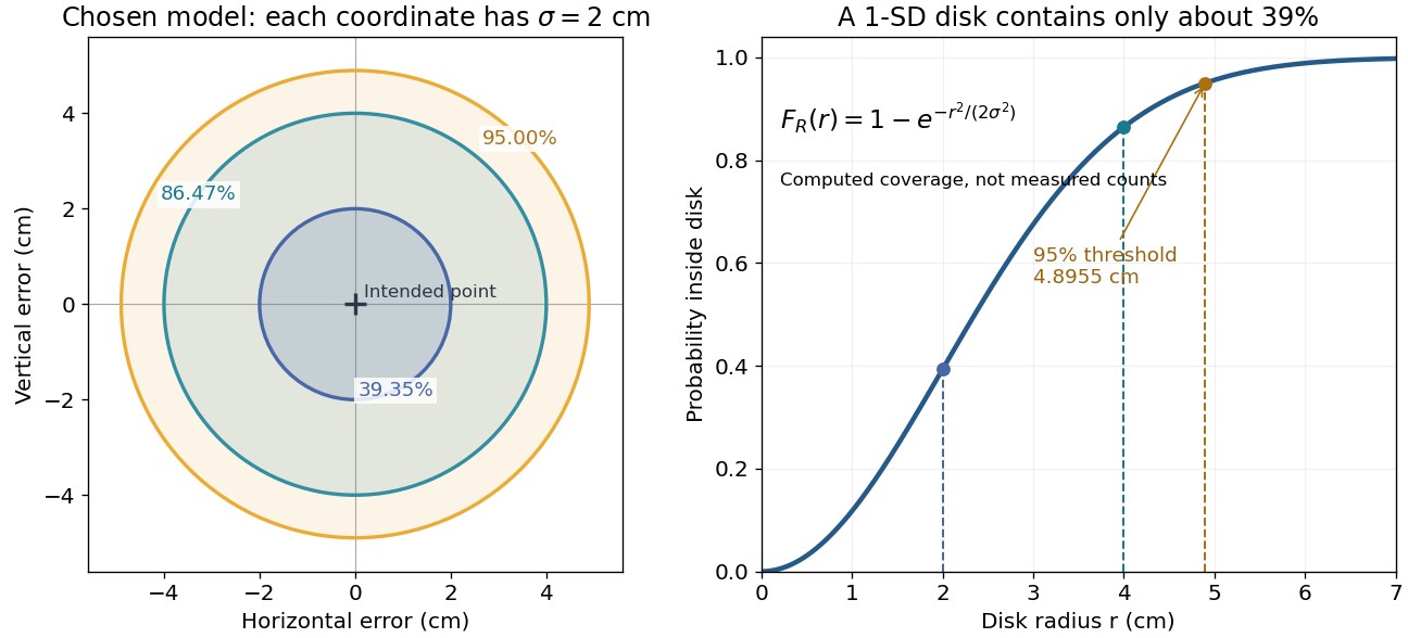
The closed-form quantile function also gives inverse transform sampling: if has uniform distribution on , then has Rayleigh distribution. Using instead gives the same law. Endpoints are excluded so that the logarithm stays finite.
The joint probability density of isIn polar coordinates, , , and the absolute Jacobian determinant is . Thus the joint density of radius and angle factors asIntegrating over angle gives the Rayleigh distribution. The same factorization shows that the angle has uniform distribution and is independent of the radius. This is a short change of variables argument: an annulus of width has area to first order.
The assumptions are substantive. Unequal component variances give elliptical rather than circular density contours; a nonzero mean displaces the center. Even zero covariance and equal normal distributions do not suffice without independence. For an original counterexample, let and let be an independent Rademacher random variable. Put . Then has the same normal distribution as , and . Nevertheless, all points lie on or , and has densitywhich is positive at zero, unlike the Rayleigh distribution. This pair is not a Gaussian random vector.
Let , with . The equation is the linear system , a rank-one matrix update of the identity matrix. Every solution has . Substitution reduces the entire problem toIf , there is one solution, . If and , every works and the solution set is the straight line . If and , there is no solution.
The first reduction follows directly from the original equation in any dimension. In three dimensions it can also be obtained by taking the cross product with , giving . The singular denominator therefore represents two different possibilities, inconsistency or a family of solutions, and must not simply be discarded as an undefined formula.
Suppose and , and is an analytic function on a disk of radius strictly larger than . The Taylor series at zero of has radius of convergence . Its coefficients are the sum of and the more rapidly decreasing coefficients of . At , the logarithmic part is an alternating harmonic series and converges conditionally; at it diverges. The power series for converges absolutely at both endpoints and therefore cannot change either conclusion. The real convergence interval is .
For , take and , with its branch normalized by . The quotient has nonzero removable value at . Its next zeros are at , so a holomorphic logarithm exists on a larger disk. This shows why the Taylor series converges at even though its singular positive endpoint is excluded.
Radius of a Maclaurin series from successive derivatives by Codex 0 Created 2026-10-18 Updated 2026-10-25
Codex 0 Created 2026-10-18 Updated 2026-10-25Write the Maclaurin series coefficients as . When the successive ratios exist eventually and have a limit, the ratio test gives the displayed radius of convergence, including zero and infinity. The unconditional formula is , from the Cauchy-Hadamard theorem. Endpoints must be checked separately.
The existence and convergence of this power series do not by themselves imply that it equals : equality requires analyticity or control of the Taylor remainder. The smooth function for , , has all derivatives zero at zero, so its Maclaurin series is identically zero despite the nonzero values away from zero.
A complex visibility is a calibrated complex correlation of the signals received at a particular interferometric baseline. In a narrow field, with scalar radiation, the far-field approximation for an outgoing source, a narrow frequency channel, negligible noncoplanar phase curvature and a steady sky of mutually incoherent emitters,Here are small dimensionless sky-direction offsets, is brightness in the chosen channel, and is the primary beam. This is the Fourier transform of beam-weighted brightness. The two-dimensional formula requires those approximations: a wide field generally needs the third baseline coordinate and curved sky geometry.
For an explicit one-dimensional derivation, set the primary beam to one over the small field, and place independent emitters at angular offsets . Choose a wave phase convention in which, after removing the phase centre's delay, their received complex amplitudes areHere is the Kronecker delta and angle brackets denote an expected value estimated by time averaging a steady signal. The last equality states mutual incoherence: different emitters have zero averaged cross term, although each emitter's two received copies remain correlated. Multiplying and averaging givesFor continuous brightness this becomes . Real brightness implies the Hermitian symmetry ; it does not require brightness to be even. In particular, an asymmetric real source usually has a nonzero imaginary complex visibility. At zero baseline, is the total beam-weighted source strength. Ordinary separated-element correlations need not measure that zero-baseline value.
Radio interferometer calibration estimates instrumental and propagation effects that alter a complex visibility. A simple narrow-field model iswhere are complex receiver gains and represents additive noise. A point-like astronomical source of known position and stable strength constrains these gains: its expected complex visibility has a known wave phase and amplitude. A resolved or variable reference source requires a better source model. Errors in the reference model can be transferred into the inferred sky.
In a proposed extension, Martin Ryle described simultaneous observation of a nearby reference point source to correct atmospheric wave phase errors, using an additional dish at each element. He presented this as a possible extension, rather than the standard One-Mile Telescope arrangement.[ref]
Radio Telescopes of Large Resolving Power by Martin Ryle. Ryle (1974), p. 202: proposed reference-source correction
An interferometric baseline is the displacement between two antennas. For a unit line of sight toward the phase centre, its projection onto the plane of the sky isHere is the speed of light. The signed delay depends on which receiver is delayed; the geometric path difference's magnitude does not. If is a unit tangent in the direction being imaged, the dimensionless coordinate is a spatial frequency, measured in cycles per radian of small sky offset. A single pair gives fringes of angular period along that tangent. This period specifies one measured oscillation; it does not specify a whole image's angular resolution or eliminate ambiguous source arrangements.
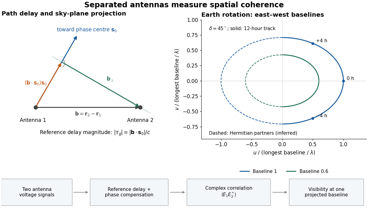
Geometric delay, projected baseline, and a schematic Earth-rotation track; original geometry, not telescope data
. Details. The left panel separates the component producing the reference delay from the component measuring angular structure. The right panel shows a possible Earth-rotation aperture synthesis track, with its opposite complex conjugate track. Those opposite samples provide the symmetry required by a real brightness distribution; they are not independent extra observations.
The phase centre is the reference sky direction for removing geometric delay and its associated wave phase. An unresolved source exactly there ideally has constant complex visibility after calibration; a displaced source has a baseline-dependent wave phase.
On a shell with homogeneous Dirichlet boundary conditions, put and . The radial heat equation in three dimensions becomes , with zero values at both endpoints. Expanding in a Fourier sine series gives the displayed solution, with . Each radial mode decays at the square of its wave number. The positive inner radius makes division by harmless throughout the shell.
For a classical monatomic homogeneous fluid with pairwise central pair potential , the mean interaction energy is one half the sum over neighbours of a tagged particle. Using the radial distribution function gives the displayed formula; the factor one half prevents counting each pair twice. The kinetic term follows from the equipartition theorem. Its use requires the relevant integral to exist and a thermodynamic state specified by number density and temperature. Quantum kinetic contributions, many-body forces and internal molecular modes require modifications.
For a differentiable central pair potential in a classical homogeneous three-dimensional fluid, the mechanical virial theorem gives the displayed pressure. The radial distribution function accounts for the probability of each pair separation. In the dilute limit, , and integration by parts yields . Thus the second virial coefficient controls . A few virial terms are a low-density approximation, not generally a converged description of a dense liquid. A discontinuous hard core needs its contact form or a limiting argument.
A constituent quark mass is an effective mass parameter in a low-energy constituent-quark model. It accounts approximately for strong-interaction dressing and some spin-independent bound-state dynamics; it is not identical to a renormalized quark mass in the Standard Model Lagrangian.
The position uncertainty of a quantum state is the standard deviation of its measured position, provided the second moment is finite. It is computed from the position operator with the Born rule. An oscillator coherent state has independently of its mean position; translating the state changes the mean without changing this variance.
If a single approximately stationary emitting region changes coherently through a causal disturbance, a disturbance travelling no faster than the speed of light takes at least to coordinate a scale . Light-travel differences also smear simultaneous emission from different depths. Under those assumptions, observed intrinsic variability on a time scale suggests .
For a chosen example , multiplication by gives . This is an order-of-magnitude causality bound on a coordinated emitting scale. It is not a measured stellar radius, and even the relation between and a diameter depends on geometry. A pulsar beam crossing is a geometric clock, and pulsar dispersion delay, scattering and instrumental response can broaden its observed pulse. The recurrence period, observed pulse width and intrinsic variability time must therefore be distinguished before applying the bound. Relativistically moving emitters require further arrival-time corrections.
Pinned article: Introduction to the OurBigBook Project
Welcome to the OurBigBook Project! Our goal is to create the perfect publishing platform for STEM subjects, and get university-level students to write the best free STEM tutorials ever.
Everyone is welcome to create an account and play with the site: ourbigbook.com/go/register. We belive that students themselves can write amazing tutorials, but teachers are welcome too. You can write about anything you want, it doesn't have to be STEM or even educational. Silly test content is very welcome and you won't be penalized in any way. Just keep it legal!
Intro to OurBigBook
. Source. We have two killer features:
- topics: topics group articles by different users with the same title, e.g. here is the topic for the "Fundamental Theorem of Calculus" ourbigbook.com/go/topic/fundamental-theorem-of-calculusArticles of different users are sorted by upvote within each article page. This feature is a bit like:
- a Wikipedia where each user can have their own version of each article
- a Q&A website like Stack Overflow, where multiple people can give their views on a given topic, and the best ones are sorted by upvote. Except you don't need to wait for someone to ask first, and any topic goes, no matter how narrow or broad
This feature makes it possible for readers to find better explanations of any topic created by other writers. And it allows writers to create an explanation in a place that readers might actually find it.
Figure 1. Screenshot of the "Derivative" topic page. View it live at: ourbigbook.com/go/topic/derivativeVideo 2. OurBigBook Web topics demo. Source. - local editing: you can store all your personal knowledge base content locally in a plaintext markup format that can be edited locally and published either:This way you can be sure that even if OurBigBook.com were to go down one day (which we have no plans to do as it is quite cheap to host!), your content will still be perfectly readable as a static site.
- to OurBigBook.com to get awesome multi-user features like topics and likes
- as HTML files to a static website, which you can host yourself for free on many external providers like GitHub Pages, and remain in full control

Figure 2. You can publish local OurBigBook lightweight markup files to either OurBigBook.com or as a static website.
Figure 3. Visual Studio Code extension installation.
Figure 5. . You can also edit articles on the Web editor without installing anything locally. Video 3. Edit locally and publish demo. Source. This shows editing OurBigBook Markup and publishing it using the Visual Studio Code extension. 
- Infinitely deep tables of contents:




All our software is open source and hosted at: github.com/ourbigbook/ourbigbook
Further documentation can be found at: docs.ourbigbook.com
Feel free to reach our to us for any help or suggestions: docs.ourbigbook.com/#contact