Topics (374k) Articles (387k) Users (410) Discussions (242) Comments (383) Files (13k) New article
A finite applicative expression over free variables and the combinator constants , with application associating to the left. One may instead take as the abbreviation . There is no variable binder in this syntax.
Bracket abstraction removes a free variable from a combinatory logic term. The displayed clauses are applied in that order, giving and . Under the standard lambda expansions of , the result is beta-equivalent to . The recursive translation of lambda terms therefore preserves variables and application and reflects weak equivalence, but need not preserve all beta equivalences.
The institution-issued AY 105 Lab Experiment 3: Optical aberrations by California Institute of Technology (Spring 2011 offering, Part A, pp. 2–3, 7–8) specifies a concrete optical bench: a lamp, opal diffuser and condensing optical lens illuminate a or optical pinhole; a photographic telephoto optical lens acts as a collimator, producing an approximately beam. A test optical lens sits on a rotation stage, followed by an adjustable optical microscope. The procedure establishes the on-axis image, then rotates the test optical lens a few degrees and examines the off-axis image through optical focus. It compares this readout with through-focus ray tracing at the corresponding field angles and offers a Ronchi ruling to calibrate the measuring eyepiece.
Part B (pp. 9–10) substitutes a spherical mirror of radius of curvature, with the optical microscope beside the incoming beam so the image is necessarily off-axis. It calls for measuring the field angle, calibrating the eyepiece and recording the image's length and width at minimum size. These are specified apparatus dimensions and instructions, not supplied measurement results or dimensions of the normalized figures.
A controlled extension would record images at zero and equal positive and negative field angles, repeat zero afterwards, and scan through optical focus at every setting. Keep the illuminated optical pupil and illumination fixed, recenter the optical microscope without clipping the bundle, and use its calibrated scale to separate a mere image displacement from a change in blur shape. The pure Seidel coma pupil mapping predicts reversal and linear growth; a stationary asymmetric central image instead calls for checking alignment. A focus-dependent change between perpendicular elongations suggests an astigmatism contribution. These comparisons test the model rather than assuming every off-axis flare is pure coma.
The optical pinhole has finite angular size, approximately its diameter divided by the collimator's focal length; the collimator and observing optical microscope also contribute their own optical aberrations. A broadband lamp can mix chromatic aberration with the geometric blur, and diffraction limits the smallest visible structure. A narrow spectral band, repeated field settings and a reference image help separate these effects. Consequently a measured length and width are useful checks on off-axis image formation, but they cannot by themselves determine a unique coma coefficient or recover the full point spread function.
Consider an original, explicitly normalized model of primary coma, rather than a prescription for a particular optical lens. Let be Cartesian coordinates in a circular optical pupil divided by its radius , with . Let be a signed small field angle divided by an arbitrary positive reference angle. With polar coordinates , , prescribe the wavefront errorHere is an arbitrary positive optical path difference scale, not a measured error. The cubic optical pupil dependence and linear field dependence are the classical Seidel form.[ref]
Coma aberration. Amateur Telescope Optics, §4.2, classical coma formula after equation 15 and equation 13: pupil-cubic and field-linear dependence
In the paraxial approximation, light ray direction errors follow the transverse gradient of wavefront error. For a reference sphere a distance from the exit optical pupil in a uniform image medium of refractive index , the corresponding image-error scale is . Choose image-error coordinate signs so the normalized displacement is ; reversing the convention reverses the plotted orientation. Image coordinates below are errors relative to the ideal image of this particular object point, rather than positions of different objects:The partial derivatives explain the asymmetry: opposite optical pupil points and land together, rather than on opposite sides of the ideal image. For , every is nonnegative, while can have either sign. The figures stipulate this single wavefront error, omit other optical aberrations and diffraction, and assign no instrument dimensions.
For a ring of fixed optical pupil radius , the double-angle formulas for trigonometric functions giveThus each ring maps into a circle of radius whose centre is displaced by . Doubling quadruples both sizes; for , the edge ring has centre and radius , while the half-radius ring has centre and radius . Superposing these displaced circles produces the comet-like envelope.
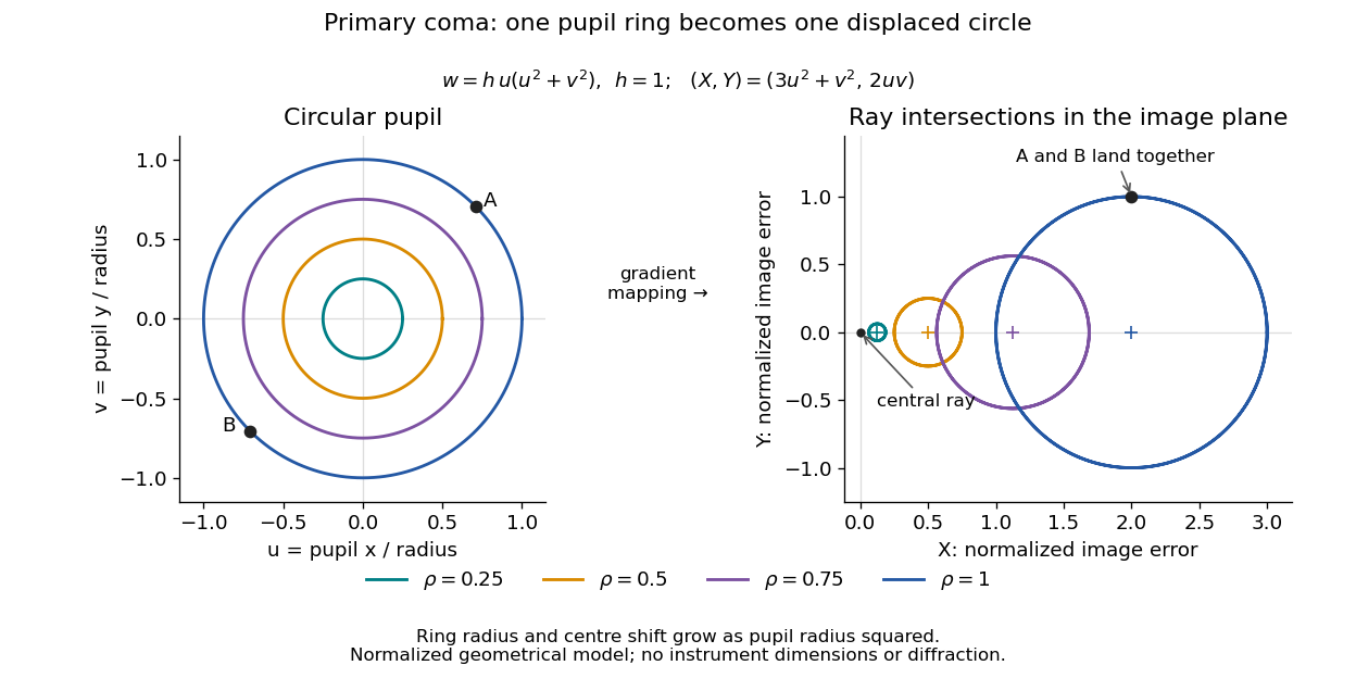
For uniform irradiance over the circular optical pupil, equal area samples give an equal-weight geometrical image. Its centroid is because and . Moving the coordinate origin to that centroid translates the image; it does not remove its asymmetric shape. Adding a linear term to likewise translates all light rays equally. These origin choices must be distinguished from changing the optical aberration itself.
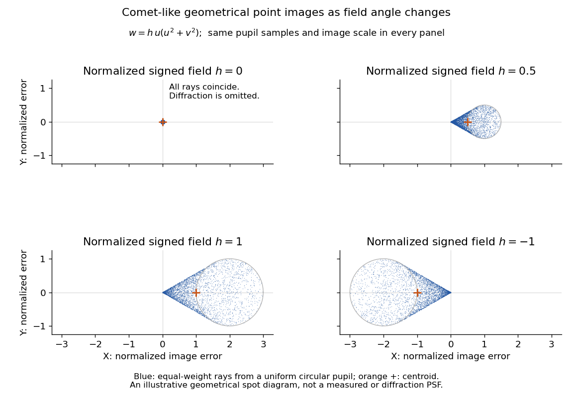
The model's full transverse extent is along and along . Halving the field angle halves the blur, and reversing it reverses the pattern about the ideal image. This isolates why coma matters for an optical camera's usable field of view: collecting more light does not ensure that off-axis points remain compact. Near diffraction-limited resolution, a physical optics calculation of the point spread function is needed instead of interpreting the geometrical tip as an infinitely sharp image.[ref]
Coma aberration. Amateur Telescope Optics, §4.2, Figure 41: geometrical spots versus diffraction images
The -stage Gauss--Legendre Runge--Kutta method collocates at the Gauss--Legendre quadrature nodes on . It is symmetric, A-stable, and has order .
For a collocation Runge-Kutta method, , where the Lagrange interpolation basis obeys . Hence each row sum is its collocation node. Failure of this identity disproves a claimed collocation tableau with those nodes. The identity alone is necessary rather than sufficient: the individual integrated basis coefficients must also agree.
For distinct collocation nodes, let . If for , and the next moment is nonzero, the associated interpolatory quadrature has order , and the collocation Runge-Kutta method has the same classical order for sufficiently smooth differential equations. Here . Equivalently, if the quadrature is exact through degree but not degree , the method has order . The generic order is at least , Gauss collocation methods reach , and Radau IIA methods reach .
For distinct nodes , the two-stage collocation Runge-Kutta method has stability functionThe denominator has no zeros in the closed left half-plane. On the imaginary axis the denominator's squared modulus minus the numerator's is . Thus , equivalently , is necessary and sufficient for A-stability, using the maximum modulus principle and the bound at infinity.
The narrow phase checks the actual objects for candidates retained by the broad phase. Its numerical guarantees depend on the chosen shape test.
// Target: analysis.bigb
The broad phase generates candidate pairs with inexpensive conservative enclosure tests. An accepted pair still needs the narrow phase.
For the negative-flux viscous Burgers equation , set . A sum of exponentials in the initial heat data evolves into , giving the displayed softmax function average. Two terms produce a traveling tanh shock from the lower to the higher state, with speed minus their mean.
Sinusoidal Cole-Hopf solution for negative-flux Burgers flow by  Codex 0 Created 2026-10-14 Updated 2026-10-18
For and initial data , the Cole-Hopf transformation gives . The Fourier series of this exponential and the heat equation give the displayed exact positive diffusion solution. Its first harmonic gives . The large-argument asymptotic expansion of a modified Bessel function makes the ratio tend to one as .
For , these sheaf cohomology dimensions follow from the vanishing for and the hyperplane exact sequence for twisting sheaves. Induct on dimension and then on in . The long exact sequence in sheaf cohomology gives higher-degree vanishing and the recurrence . Starting with yields the formula; the corresponding homogeneous monomials form a basis of global sections.
There is no fiber bundle when and is odd. A local trivialization makes a retract of an open subset of , so for ; the long exact sequence of homotopy groups of a fibration makes connected. In the multiplicative rational Serre spectral sequence, only base columns zero and occur. Since , a fibre class must satisfy , the base generator. Its degree is even. If is its first vanishing power, the derivation law gives on the page, a contradiction. Bounded fibre cohomology ensures such a vanishing power exists. In particular cannot be the total space of a bundle over .
Use the signature of unital commutative rings, its equational axioms, and the coherent sequents and , where abbreviates . In a set-based model the nonunits form its unique maximal ideal; this is the usual nonzero local ring. In a topos the disjunction expresses local existence of a unit witness. Its classifying topos is defined by the Zariski coverage on finitely presented rings.
Suppose the first ancilla records parity , then a fault of value flips , and the second ancilla records parity . For incoming bit-error pattern , the observed error syndrome is the displayed pair, while the final data error before recovery is . When , the observed syndrome differs from the actual data syndrome by . Applying the usual minimum-weight recovery leaves a nonzero syndrome, so the state is outside the code space even when the channel itself made no error. This is a timing-dependent failure of this simple extraction circuit, not a general obstruction to fault-tolerant quantum error correction.
For a block sliding right on a stationary horizontal plane, take rightward acceleration as positive. A gauge reading for a pull at angle above horizontal has horizontal component and upward component . With no vertical acceleration or other forces, Newton's second law givesand thereforeThis inference requires continued contact with and rightward contact slip, so its numerator must be nonnegative. An upward pull reduces normal force; a downward pull, represented by , increases it. The horizontal constant-velocity formula is the special case , .
For the original , model, an upward pull at maintaining constant velocity needsDividing this gauge reading by would give about , rather than : the gauge reads the full inclined force, and the pull has changed the normal force.
Even with a horizontal pull, an accelerating measurement needs the correction: . In the same model, a horizontal pull produces while the block slides right; subtracting recovers the kinetic friction. Dividing the uncorrected reading by instead gives about . Measure acceleration in an inertial frame, along the sliding direction, over the same interval as the gauge reading. These corrections follow from the force balance, independently of whether the resulting coefficient of kinetic friction is constant across runs.
// Target: classical-mechanics.bigb
Changing the added mass while retaining the same contact pair and sliding speed tests whether a constant coefficient of kinetic friction is a useful model. Compute for each level horizontal run, and plot the mean sliding force vertically against normal force horizontally. The constant-coefficient prediction is a straight line through the origin; its slope is . This extracts a ratio from several loads rather than relying on one reading.
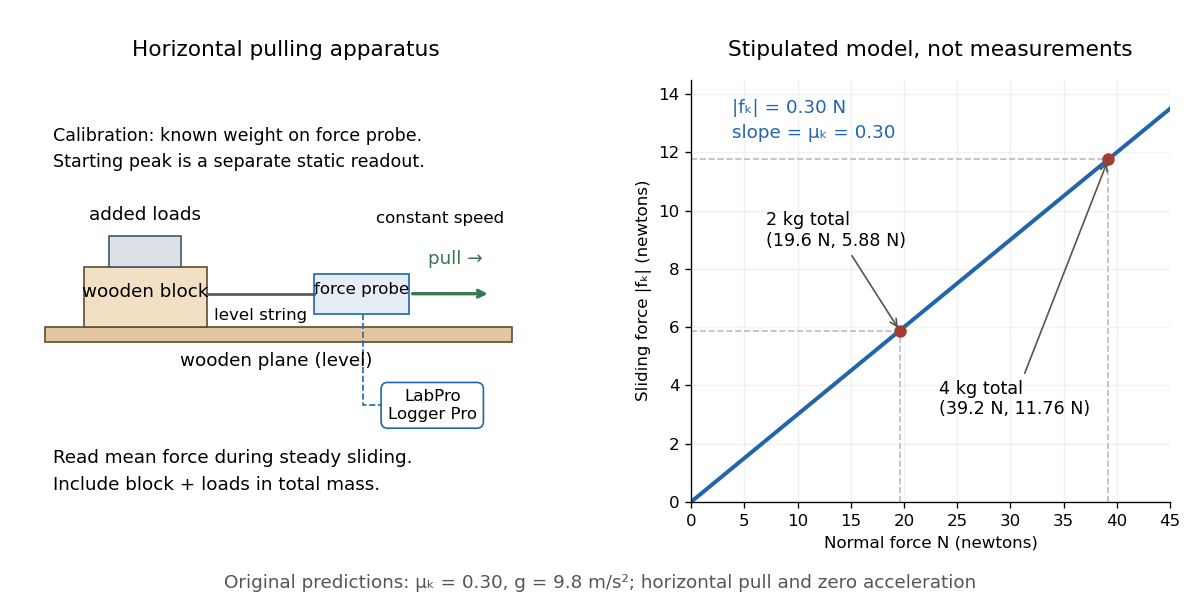
Horizontal wooden-block force-probe apparatus and original load model: 19.6 N and 39.2 N normal loads predict 5.88 N and 11.76 N sliding forces
. Details. The apparatus sketch identifies the contact pair and horizontal pull used by the cited laboratory procedure. The plotted line and points are the original stipulated model from coefficient of kinetic friction, not laboratory data. The two model points giveIn actual measurements, a linear regression can expose an unexplained intercept . A nonzero intercept calls for checking the gauge zero, other resisting forces and the contact model; forcing the line through zero can hide those problems. Conversely, constant ratios within measurement error support the approximation only over the loads, speeds and surface conditions tested. A load sweep alone cannot establish independence from contact area or sliding speed; those require separate controlled variations.
A force gauge reads the pulling force. For horizontal straight-line sliding at constant velocity, its reading equals the opposing kinetic friction magnitude, provided these are the only horizontal forces. For total supported mass , including added loads, , so a mean sliding reading gives . The important readout is the sustained sliding force after the starting peak; the peak belongs to the static friction threshold.
The University of Mississippi's Experiment 6 uses a wooden block on a wooden plane, a triple-beam balance, added masses, and a dual-range 50 N force probe connected through LabPro to Logger Pro. Its procedure calibrates the probe with a load on a hanger, entering the corresponding force in newtons, and measures the block's mass separately. With the plane horizontal, it starts with on the block and pulls horizontally at constant speed. The recorded force trace has a starting peak; the procedure selects the subsequent constant-force interval and takes its mean. It repeats with increments up to added, then plots sliding force against normal force to estimate the coefficient of kinetic friction from the slope.[ref]
Experiment 6: The Coefficient of Friction (University of Mississippi teaching laboratory). Experiment 6, The Coefficient of Friction, PDF pp. 1–2: Equipment, Objectives, Procedure steps 1–7
For a replication, check the gauge's zero with the string slack and its response to known gravitational weights; zeroing alone does not check its scale. Keep the plane level, the pull parallel to it, and the block face and track region consistent. Specify the contacting materials and whether the surfaces are dry, cleaned or lubricated; repeat runs to see whether debris or wear changes the sliding force. Verify constant velocity independently from position versus time, rather than assuming that a flat force trace proves zero acceleration. These are proposed measurement controls, not additional observations from the laboratory writeup. Record the selected interval, variation between runs and gauge resolution as sources of measurement error.
In the standard genetic code, UAA, UAG and UGA are stop codons: they signal termination of biological translation rather than an amino acid assignment. See Clark, Douglas and Choi: stop codons.
A stop codon supplies no additional amino acid residue. In the constructed AUG GCU UUC UGA example, replacing UGA by UAA preserves termination after the same three amino acid residues. Replacing UUC by UAA instead terminates after methionine and alanine. These are consequences of the stated genetic code, not measurements of expression efficiency.
At a standard stop codon, a release factor promotes release of the polypeptide from the ribosome. Ordinary delivery of an amino acid by transfer RNA does not supply a “stop amino acid”.[ref]
Biology 2e by Mary Ann Clark and others. §15.5, Translation, Elongation, and Termination, paragraph beginning “Termination of translation”: stop codons and release factors
Pinned article: Introduction to the OurBigBook Project
Welcome to the OurBigBook Project! Our goal is to create the perfect publishing platform for STEM subjects, and get university-level students to write the best free STEM tutorials ever.
Everyone is welcome to create an account and play with the site: ourbigbook.com/go/register. We belive that students themselves can write amazing tutorials, but teachers are welcome too. You can write about anything you want, it doesn't have to be STEM or even educational. Silly test content is very welcome and you won't be penalized in any way. Just keep it legal!
Intro to OurBigBook
. Source. We have two killer features:
- topics: topics group articles by different users with the same title, e.g. here is the topic for the "Fundamental Theorem of Calculus" ourbigbook.com/go/topic/fundamental-theorem-of-calculusArticles of different users are sorted by upvote within each article page. This feature is a bit like:
- a Wikipedia where each user can have their own version of each article
- a Q&A website like Stack Overflow, where multiple people can give their views on a given topic, and the best ones are sorted by upvote. Except you don't need to wait for someone to ask first, and any topic goes, no matter how narrow or broad
This feature makes it possible for readers to find better explanations of any topic created by other writers. And it allows writers to create an explanation in a place that readers might actually find it.
Figure 1. Screenshot of the "Derivative" topic page. View it live at: ourbigbook.com/go/topic/derivativeVideo 2. OurBigBook Web topics demo. Source. - local editing: you can store all your personal knowledge base content locally in a plaintext markup format that can be edited locally and published either:This way you can be sure that even if OurBigBook.com were to go down one day (which we have no plans to do as it is quite cheap to host!), your content will still be perfectly readable as a static site.
- to OurBigBook.com to get awesome multi-user features like topics and likes
- as HTML files to a static website, which you can host yourself for free on many external providers like GitHub Pages, and remain in full control

Figure 2. You can publish local OurBigBook lightweight markup files to either OurBigBook.com or as a static website.
Figure 3. Visual Studio Code extension installation.
Figure 5. . You can also edit articles on the Web editor without installing anything locally. Video 3. Edit locally and publish demo. Source. This shows editing OurBigBook Markup and publishing it using the Visual Studio Code extension. 
- Infinitely deep tables of contents:




All our software is open source and hosted at: github.com/ourbigbook/ourbigbook
Further documentation can be found at: docs.ourbigbook.com
Feel free to reach our to us for any help or suggestions: docs.ourbigbook.com/#contact