Topics (384k) Articles (398k) Users (410) Discussions (242) Comments (383) Files (13k) New article

With the curvature sign convention in which , the inverse-metric variation of is plus a boundary term, for a scalar multiplier held fixed in that variation. The Palatini identity expresses the curvature variation as divergences of . Two integrations by parts move the derivatives onto , yielding the displayed terms. For constant they vanish. The opposite curvature convention instead has .
For a Hermitian scalar field in a positive-norm Hilbert space with a Lorentz-invariant vacuum, the spectrum condition and completeness give the connected vacuum two-point function as a superposition of free mass-shell functions. Define the Källén–Lehmann spectral density by , where and its vacuum expectation value has been subtracted if nonzero. Squared intermediate-state matrix elements make a nonnegative measure supported on nonnegative mass squared. Applying time ordering to each free mass shell gives the displayed Feynman propagator representation, using and signature . Its positivity does not automatically extend to gauge-variant fields in an indefinite auxiliary space.
For the state-space model with both scalar coefficients equal to one, and . If the variance converges and , its limiting gain satisfies . The nonnegative root lies below one for finite ; it tends to zero with and to one as grows. Thus noisier state evolution assigns more weight to the latest observation.
For spatial scalar convention and , a passive gauge displacement gives and . Moving from synchronous gauge to Newtonian gauge therefore requires and . A scalar density transforms by , giving the displayed density contrast relation. Keeping the background lapse function explicit prevents cosmic-time and conformal-time factors from being confused.
A local minimum of the scalar potential that has higher energy than a global minimum. It can be stable against infinitesimal classical fluctuations but metastable to a transition to a lower-energy vacuum, including quantum tunnelling. The stability of a cubic-quartic scalar potential gives an elementary example distinguishing local curvature from global stability.
For , positive makes the classical potential bounded below. For , completing the square givesThus zero is a global minimum precisely when . At a nontrivial equality there are degenerate minima at zero and . If and the inequality fails, zero is a false vacuum: its Hessian is positive but another minimum has lower energy. A negative quartic coupling, or a nonzero cubic term without a quartic term, is unbounded below. These are classical or tree-level criteria.
For a differentiable scalar conservation law , a sonic point of a scalar flux is a state where its characteristic speed vanishes. If is convex and this zero is unique, on the left and on the right, so is the unique minimum of the flux. The definition refers to a vanishing transport speed in a scalar conservation law. In compressible fluid mechanics, a sonic point instead refers to flow at the local sound speed.
The saturation intensity sets the physical crossover from linear optical response to saturated excitation. For an ideal radiatively damped two-level system driven on resonance, define , where is the Rabi frequency and is the spontaneous emission rate. Its steady excited population and total photon scattering rate areAt , and : half the high-intensity scattering limit . This gives the scale an observable meaning beyond simply defining a ratio. [ref]
Rubidium 87 D Line Data by Daniel A. Steck. Section 4.2, equations 47–50, steady two-level population, scattering and saturation convention
The value depends on the transition dipole moment, driving polarization and sublevel populations. Optical pumping or extra dephasing can alter the effective response. Therefore comparisons must state the transition and illumination convention; a tabulated value for one geometry cannot automatically be assigned to another. [ref]
Rubidium 87 D Line Data by Daniel A. Steck. Equation 50 and following polarization/alignment discussion; section 4.3, optical pumping
For individual Bernoulli observations, the statistical saturated model assigns one independent probability to each response. Each likelihood factor is at most one and is exactly one at . Hence the maximum log-likelihood is zero, with . This boundary maximum is attained when probabilities zero and one are allowed; restricting them to the open interval gives the same supremum.
In a countable language, an ultraproduct over a nonprincipal ultrafilter on realizes every countable finitely satisfiable type, including types over countably many parameters. Enumerate the type , and let be the ultrafilter-large set of coordinates where the first first-order formulas have a simultaneous witness. Put . At coordinate , choose a witness for the largest with , or an arbitrary element when there is none. For each fixed , the resulting function satisfies the first first-order formulas on . The Łoś theorem then realizes the entire type. Countability of the language and parameter set makes the enumeration possible.
For every infinite regular cardinal , every first-order structure has a -saturated elementary extension. At one stage use the compactness theorem with the elementary diagram to realize all complete types over subsets of the stage having size less than . There is a set of such types; finite subsets of the enlarged theory are satisfiable because their finitely many witnesses are independent. Iterate for stages, taking elementary unions at limits. Regularity puts any parameter set of size less than inside one stage, and its type is realized at the next one. Passing to a larger regular cardinal covers singular requested degrees of saturation as well.
Suppose satisfies the mixed domination on a subspace , and . Apply that domination to and , split the argument as , and use superadditivity of . This proves every lower candidate in the displayed interval is at most every upper candidate. The zero-vector candidates bound the lower supremum below by and the upper infimum above by , so both endpoints are finite. Choosing any intervening value permits . For , scale the upper comparison by ; for , scale the lower comparison by . Both give the required mixed domination, proving the interval characterizes the permitted extension values.
When items among are marked, inspect a uniformly random permutation until the first marked item. For its first position to be , the other marked positions must lie among the last slots. This yields the displayed law with support . It is the first-success form of sampling without replacement. For one marked item the position is uniform, while its conditional success chance after failures increases to .
For two independent normal samples of sizes with a common unknown variance, pooling their within-sample sums of squares gives the unbiased estimator . The numerator divided by the common population variance has a chi-squared distribution with degrees of freedom and is independent of both sample means. Therefore has a Student t-distribution. This exact construction requires a positive residual number of degrees of freedom and the common-variance assumption.
The empirical variance is the variance of the empirical distribution, which puts probability on each observation. It uses divisor , whereas the usual sample variance uses divisor . For independent and identically distributed random variables with finite second moment, jackknife bias correction converts the empirical variance into the unbiased estimator exactly.
Model two fair independent coin tosses, recording their order. Here denotes heads and tails, andThe power set includes every question expressible as a subset of these four outcomes. The mass comes from the fairness and independence assumptions. These are exact model probabilities, rather than measured toss frequencies.
Let be the event that the first toss is heads and the event that the second toss is heads. ThenThe union means “at least one head,” while the intersection means “both heads.” Their probabilities are and . Counting the union through the inclusion-exclusion principle gives ; alternatively its complement of an event is , of probability .
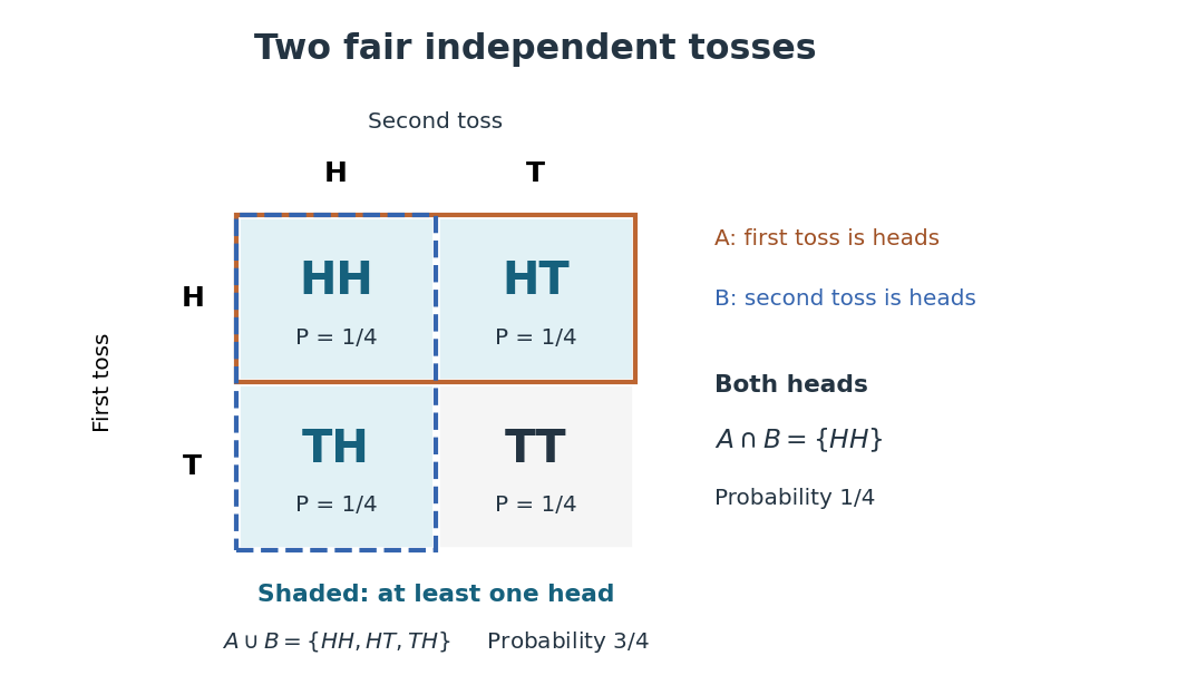
Four ordered outcomes and the event of at least one head
. Rows record the first toss and columns the second. Each cell has probability under fair independent tosses. The highlighted union includes , , and ; the overlap contains only . Details.On the same sample space, assigning masses to would still make each toss fair: . But , so the tosses would be dependent. The event of at least one head would have probability . Changing the probability measure changes the answer even when the sample space and the single-toss probabilities stay the same.
An elementary outcome is one member of the sample space. For the ordered two-toss model, is one outcome; it contains both toss results. By contrast, “at least one head” is an event containing three outcomes. The outcome and the singleton set are different objects: when that singleton is measurable, the notation gives its probability. In the finite model below, every subset is measurable.
The word elementary refers to the chosen level of detail. An outcome can be an ordered pair, a sequence, or an entire realization of a point process. A random variable then extracts a numerical feature of that outcome; the window count of a point process is one example.
A sample size calculation for a binary endpoint requires its own baseline probability, not merely the rate of a related outcome. A fatal-event probability equals the probability of the underlying event times its conditional fatality probability; knowing only that product does not identify the incidence of all events. Thus a mortality rate can size a mortality trial but cannot determine the size for all fatal and nonfatal events without further assumptions. The significance level, allocation, target statistical power and effect definition must also be specified.
Suppose each collaborating centre contributes independently randomized participants per arm with specified event probabilities. At 50% statistical power, the usual normal-approximation alternative quantile is zero. The required size per arm is , with for a two-sided test or for a one-sided test. Divide by the per-centre arm size and round up. Endpoints must use the same time origin and follow-up window, and cluster dependence requires an additional adjustment.
Pinned article: Introduction to the OurBigBook Project
Welcome to the OurBigBook Project! Our goal is to create the perfect publishing platform for STEM subjects, and get university-level students to write the best free STEM tutorials ever.
Everyone is welcome to create an account and play with the site: ourbigbook.com/go/register. We belive that students themselves can write amazing tutorials, but teachers are welcome too. You can write about anything you want, it doesn't have to be STEM or even educational. Silly test content is very welcome and you won't be penalized in any way. Just keep it legal!
Intro to OurBigBook
. Source. We have two killer features:
- topics: topics group articles by different users with the same title, e.g. here is the topic for the "Fundamental Theorem of Calculus" ourbigbook.com/go/topic/fundamental-theorem-of-calculusArticles of different users are sorted by upvote within each article page. This feature is a bit like:
- a Wikipedia where each user can have their own version of each article
- a Q&A website like Stack Overflow, where multiple people can give their views on a given topic, and the best ones are sorted by upvote. Except you don't need to wait for someone to ask first, and any topic goes, no matter how narrow or broad
This feature makes it possible for readers to find better explanations of any topic created by other writers. And it allows writers to create an explanation in a place that readers might actually find it.
Figure 1. Screenshot of the "Derivative" topic page. View it live at: ourbigbook.com/go/topic/derivativeVideo 2. OurBigBook Web topics demo. Source. - local editing: you can store all your personal knowledge base content locally in a plaintext markup format that can be edited locally and published either:This way you can be sure that even if OurBigBook.com were to go down one day (which we have no plans to do as it is quite cheap to host!), your content will still be perfectly readable as a static site.
- to OurBigBook.com to get awesome multi-user features like topics and likes
- as HTML files to a static website, which you can host yourself for free on many external providers like GitHub Pages, and remain in full control

Figure 2. You can publish local OurBigBook lightweight markup files to either OurBigBook.com or as a static website.
Figure 3. Visual Studio Code extension installation.
Figure 5. . You can also edit articles on the Web editor without installing anything locally. Video 3. Edit locally and publish demo. Source. This shows editing OurBigBook Markup and publishing it using the Visual Studio Code extension. 
- Infinitely deep tables of contents:



All our software is open source and hosted at: github.com/ourbigbook/ourbigbook
Further documentation can be found at: docs.ourbigbook.com
Feel free to reach our to us for any help or suggestions: docs.ourbigbook.com/#contact