A wetting liquid penetrates pore space under a pressure difference that includes capillary suction. With a planar front, fixed pressure drop and negligible gravity/inertia, Darcy's law and pore-volume storage give $z\propto t^{1/2}$. The front pressure must be defined relative to the gas phase consistently; adding a positive suction to the inlet pressure is different from prescribing a positive liquid front pressure.

Without transverse exchange, a particle chosen uniformly from pore volume samples each streamline's transit time with resident-volume weight. This differs from the flux-weighted residence time in a porous layer, which samples at the inlet proportionally to $v$. For constant porosity and a linear positive velocity $v=v_0+(v_1-v_0)y/H$, the two means are $L\log (v_1/v_0)/(v_1-v_0)$ and $2L/(v_0+v_1)$, respectively. Their limits agree for uniform velocity.

For a nonzero multivariate polynomial of total degree $d$ over a field, and a finite subset $S$ of that field, at most $d|S{|}^{n-1}$ points of $S^n$ are zeros. For one variable this is the root bound for a polynomial. If $d\ge |S|$, the bound is already trivial. Otherwise, in the inductive proof write the polynomial as degree $k$ in its last variable, with a nonzero leading coefficient of degree at most $d-k$ in the other variables. The leading coefficient vanishes on at most $(d-k)|S{|}^{n-2}$ fibers; outside those fibers there are at most $k$ roots of a polynomial per fiber. Counting the bad fibers with the trivial $|S|$ bound gives the asserted inequality.

Suppose every point of ${\mathbb{F}}_q^n$ lies on an affine line in a vector space meeting a subset $N$ in at least $m$ points, with $1\le m\le q$. A smaller $N$ would admit a nonzero multivariate polynomial of total degree at most $m-1$ vanishing on it, by the dimension of a bounded-total-degree polynomial space. Each selected line then has more roots of a polynomial than the degree of its restriction, so the polynomial vanishes at every point. The Schwartz-Zippel lemma forbids this because $m-1<q$. Thus the displayed bound holds, and is at least $m^n/n!$. This is a point-covering condition; the finite-field Kakeya set condition instead quantifies over directions.

An asteroid is a small rocky or metallic body orbiting a star. Asteroid dynamics can involve mean-motion resonances, planetary scattering and secular perturbations. Solar-system asteroids illustrate how phase protection can prevent close encounters even when orbital paths approach a planet.

For the orthonormal coframe of a planar warped spacetime, Cartan's first structure equation gives ${\omega }^i{}_3=a{e}^i$ and ${\omega }^3{}_i=-s_{i}a{e}^i$, where $i=0,1,2$ and $(s_0,s_1,s_2)=(-1,1,1)$. All other connection 1-forms vanish. Cartan's second structure equation gives ${\Theta }^i{}_3=-q{e}^i\wedge e^3$ and ${\Theta }^i{}_j=-s_j{a}^2{e}^i\wedge e^j$ for $i\ne j$. Lowering the first index makes both the connection 1-forms and the curvature 2-forms antisymmetric. Contraction yields $R_{00}=q+2a^2$, $R_{11}=R_{22}=-q-2a^2$, and $R_{33}=-3q$.

For a real on shell photon of null momentum $k$, a physical polarization satisfies $k\cdot ϵ=0$ and is defined modulo $ϵ\mapsto ϵ+\alpha k$. The two-dimensional quotient carries the two physical photon helicities. In a transverse gauge choose ${ϵ}^0=0$ and ${ϵ}^{\ast }\cdot ϵ=-1$. A Ward identity ensures that replacing an external polarization by its momentum gives zero in the summed physical amplitude.

Absorption of an ionizing photon leaves energy in a photoelectron above the binding energy. Thermalization supplies heat to the gas. Photoionization heating competes with the astrophysical cooling function, can establish thermal equilibrium, and can raise the pressure enough to inhibit baryon accretion into shallow dark-matter haloes.

A cyclic ordering of a finite ground set records its elements around an oriented circle, identifying permutations that differ by rotation. There are $(n-1)!$ such orderings for $n\ge 1$. A uniformly random permutation induces a uniformly random cyclic ordering.

Thermokarst is subsidence and related landscape change caused by thaw of ice-rich permafrost. Resulting lakes and saturated sediments can promote methanogenesis.

A Gaussian auxiliary-field identity replacing a quadratic expression in a composite field by a linear coupling to a new field. Completing the square in $M^2/(2U)-Mj$ yields an exponential $e^{U{j}^2/2}$ after integrating $M$, with normalized Gaussian prefactors. It converts suitable quartic field interactions into bilinear couplings and permits fermionic fields to be integrated out.

A quadratic path integral becomes a product of Gaussian integrals after diagonalizing its fluctuation operator. One real coordinate per mode gives an inverse square root of the functional determinant; one complex coordinate, or two real coordinates, gives its inverse. A regulator and normalization are essential: determinant ratios are often meaningful before an absolute determinant is defined.

For a Hamiltonian operator with kinetic term ${\hat{p}}^2/2$, insert position-basis resolutions between Trotter product formula factors. The measure is the limit of $(2\pi i\Delta {)}^{-M/2}{\prod }_{j=1}^{M-1}d{q}_j$, and the exponent contains ${\sum }_j[(q_j-q_{j-1}{)}^2/(2\Delta )-\Delta V(q_{j-1})]$. Its continuum notation is $\int \mathcal{D}q{e}^{iS[q]}$, with fixed endpoint values. A damping prescription defines the oscillatory limit.

For a radiation-filled expanding universe with $0<{\Omega }_0<1$ and no cosmological constant, set $x=a/a_0$. The particle horizon radial proper distance is $H_0^{-1}{\int }_0^1[{\Omega }_0+(1-{\Omega }_0)x^2{]}^{-1/2}dx$. An inverse-hyperbolic-sine antiderivative gives the formula. The spatially flat limit is $d_{h0}=H_0^{-1}$; radial proper distance is distinct from the area radius of the corresponding horizon sphere.

The Pareto frontier consists of feasible payoff vectors that no other feasible vector weakly improves in every coordinate and strictly improves in at least one. A Nash bargaining solution with positive gains lies on this frontier, because increasing either gain without decreasing the other raises its Nash product.

For a homogeneous harmonic polynomial $H_l$ of degree $l$ in three dimensions, the Euler theorem for homogeneous functions gives $D{H}_l=l{H}_l$, where $D=\mathbf{x}\cdot \nabla$. The orbital angular momentum identity ${\hat{L}}^2=-{\hslash }^2(r^2\Delta -D^2-D)$ therefore gives ${\hat{L}}^2{H}_l=l(l+1){\hslash }^2{H}_l$. This constructs angular momentum eigenstates directly from polynomials.

A stochastic control problem chooses an admissible control input using information available in a filtration to optimize an expected objective for a random dynamical system. Dynamic programming often characterizes its value function through a Hamilton-Jacobi-Bellman equation.

Interval bisection solves a target equation $f(x)=t$ by repeatedly halving a closed interval known to contain a solution. It is the bisection method applied to $g(x)=f(x)-t$, so the target becomes a zero of a function. This reduction from an equation to root finding is described in Demanet's notes.^[ref] Here the emphasis is on a continuous strictly increasing function: the target identifies one input, making interval bisection a way to evaluate its inverse function without an explicit inverse formula.

Let $f:[a_0,b_0]\to \mathbb{R}$ be a continuous function, with $a_0<b_0$ and $f(a_0)\le t\le f(b_0)$. The intermediate value theorem guarantees existence; a strictly increasing function also guarantees uniqueness. Check endpoint equality first. Otherwise, for the current root bracket $[a_k,b_k]$, evaluate its midpoint $m_k=(a_k+b_k)/2$. If $f(m_k)<t$, retain $[m_k,b_k]$; if $f(m_k)>t$, retain $[a_k,m_k]$; if $f(m_k)=t$, return that exact solution. These comparisons preserve the target bracket. General bisection method needs continuity and opposite signs of $g$ at the endpoints, without requiring monotonicity or a unique zero of a function; see limitations of bisection.

An original dimensionless polynomial example isHere $f(0)=0<10<30=f(3)$ and the derivative $f^{\prime }(x)=3x^2+1>0$, so there is exactly one solution. In fact $x_{\ast }=2$; knowing this lets us check the computed absolute error independently of the guarantee. The first four halvings give the following exact rational numbers:

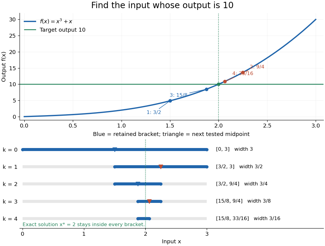
The beauty of interval bisection is that the enclosure itself supplies the certificate: one comparison removes half the possible inputs, regardless of the steepness of the function graph. In exact arithmetic, after $k$ completed halvings without exact termination, the width and the bisection error bound for the new midpoint areThe reported midpoint after update four is $m_4=63/32$, rather than the last tested point $m_3=33/16$. Its certified absolute error is at most $3/32$, and its actual absolute error is $1/32$. For a requested position tolerance $10^{-3}$, the bisection stopping criterion requires eleven halvings: ten give $3/2048>10^{-3}$, while eleven giveThe actual absolute error is $1/4096$. The new midpoint need not be evaluated to obtain this certificate.

The signed output residual is $r=f(m)-t$; the position approximation error is $m-x_{\ast }$. They answer different questions: how close is the output to the target, and how close is the input to the solution? Driscoll and Braun explain why a small residual needs information about the derivative to imply small position error.^[ref] For this particular polynomial, direct factorization givesThus at $m_4=63/32$ the residual is $-13121/32768\approx -0.400421$, despite position absolute error $1/32=0.03125$. If a differentiable function satisfies $0<\ell \le f^{\prime }(x)\le L$ throughout the bracket, the mean value theorem gives the rigorous conversionOur example permits $\ell =1$ and $L=28$ on $[0,3]$. Strict increase alone supplies no positive lower derivative bound: $f(x)=x^3$ is strictly increasing but $f^{\prime }(0)=0$. A small residual alone is therefore not a universal position certificate; even the target equation $10^{-6}(x-2)=0$ has residual $10^{-6}$ at $x=3$, a full unit from its solution.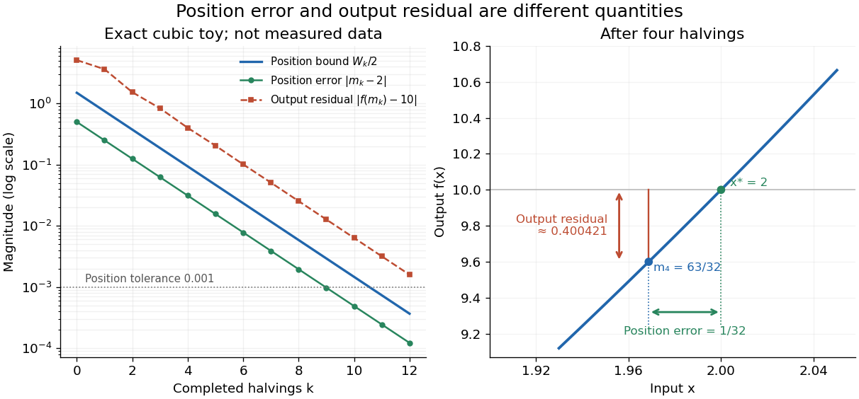

The guarantees require continuity and correct evaluations, not just narrowing endpoints. For the strictly increasing function $h(x)=x$ when $x<0$ and $h(x)=x+1$ when $x\ge 0$, the target $1/2$ lies between $h(-1)$ and $h(1)$ but is never attained: a jump discontinuity defeats the existence argument. With floating-point arithmetic or an approximate evaluation, an incorrect comparison can discard the true solution. A certified interval enclosure of $f(m)$ wholly below or above $t$ certifies the corresponding decision; an enclosure containing $t$ is inconclusive, rather than proof of equality. If rounding makes the midpoint equal an endpoint, report the precision limit; see bisection stopping criterion for the rounded position bound. Both figures are exact mathematical examples, not measured data.

The finite volume method follows the amount of a conserved quantity inside each control volume. Its unknowns are cell averages, rather than values at isolated points: a cell's width times its stored average approximates that cell's total. A numerical flux transfers an amount across a face. Using one shared transfer for both neighboring cells makes the loss from one exactly the gain of the other, as explained in shared face flux cancellation.^[ref]

For a one-dimensional scalar conservation law without sources, let $u_t+{\partial }_{x}f(u)=0$, with conservation law flux $f$. Fix cells $I_j=[x_{j-1/2},x_{j+1/2}]$ of widths $h_j>0$. Define the exact cell average and its numerical approximation byThe integral balance over one cell and one time interval of length $k>0$ isFor a smooth solution this follows by integration of the differential equation; with jump discontinuities, it expresses the conservation law in integral form, using appropriate face traces when they exist. Replacing each time-averaged face conservation law flux by a numerical flux givesThus the finite volume method implements a balance directly, without needing a pointwise derivative at a jump. The tube balance in Riemann Problems and Jupyter Solutions by David I. Ketcheson, Randall J. LeVeque, and Mauricio J. del Razo (Advection, §Conservation of mass) motivates this construction from conservation of mass.

This is useful for shock waves: their speed is constrained by the Rankine-Hugoniot condition, itself an integral balance. A nonconservative approximation can give a visibly plausible jump with the wrong speed. Conservation is one requirement; a nonlinear scalar conservation law also needs the correct entropy solution, and the chosen numerical flux and update need their own stability and accuracy analysis.^[ref] The original periodic upwind finite volume advection example isolates the shared-transfer mechanism in a problem with a known translated solution.

Suppose a ring has an underlying real normed vector space and its norm is multiplicative, without initially assuming real bilinearity of multiplication. For fixed $x$, distributivity makes $y\mapsto xy$ additive, while $\Vert xy-xz\Vert =\Vert x\Vert \Vert y-z\Vert$ makes it continuous. Additivity gives rational scalar compatibility, and continuity extends it to every real scalar. Apply the same argument in the other variable to obtain a bilinear map. The norm identity also excludes nonzero zero divisors.