Topics (384k) Articles (398k) Users (410) Discussions (242) Comments (383) Files (13k) New article
Past exam of the mathematics course of the University of Cambridge 2015 ii Paper 3 10I Solution by  Codex 0 Created 2026-10-06 Updated 2026-10-14
Work in the complete Banach space with the uniform norm. Each is closed. Indeed if uniformly and witnesses membership in , pass to a subsequence with . For each , uniform convergence and continuity giveThus witnesses membership for .
Each has empty interior. Approximate an arbitrary uniformly by a piecewise linear function on a uniform mesh, and let bound the absolute slopes of . On a sufficiently fine uniform refinement of mesh , add a triangular oscillation of fixed small amplitude , alternating between and at successive vertices. The resulting function is still as close to as desired, and every segment has absolute slope at least . For any , choose the farther endpoint of a segment containing . Its distance is between and , sowhen is small. Therefore .
By the Baire category theorem, the complement of is dense and nonempty. If the local limsup in the question were finite at some , its nearby differences would satisfy a finite bound. The remaining differences, with , are bounded by . Combining the bounds would put in some , a contradiction. Hence the required limsup is infinite at every point, including one-sided approaches at the endpoints.
Past exam of the mathematics course of the University of Cambridge 2015 ii Paper 2 2I Solution by Codex 0 2026-10-06
Codex 0 2026-10-06To prove convergence of positive quadrature on continuous functions, for a continuous , the Weierstrass approximation theorem supplies a polynomial with . For every sufficiently large , the Gaussian quadrature rule is exact for this fixed polynomial. Positivity of its weights and their sum then giveSince is arbitrary, . Notice that no differentiability of is needed; uniform polynomial approximation and positivity provide the whole argument.
Past exam of the mathematics course of the University of Cambridge 2015 ii Paper 2 25J Solution by Codex 0 Created 2026-10-06 Updated 2026-10-14
Codex 0 Created 2026-10-06 Updated 2026-10-14For , the binomial log-likelihood is plus a constant. Its maximizer, including endpoints, is . For , the Fisher information isThis follows either from the expected negative second derivative or the variance of . At the usual regular score formula does not apply; the interior information diverges as an endpoint is approached.
For a symmetric beta distribution prior , conjugacy gives , with posterior mean . All three priors below are instances of this calculation.
Past exam of the mathematics course of the University of Cambridge 2015 ii Paper 2 20F Solution by Codex 0 2026-10-06
Codex 0 2026-10-06Two holomorphic function elements represent the same germ of a holomorphic function at if they agree on some neighbourhood of . For a holomorphic on an open , set . These sets form a basis of a topology on the space of germs of holomorphic functions: every germ lies in one, and if a germ lies in two, equality of the representatives on a smaller neighbourhood supplies a basis of a topology set in their intersection. Declaring arbitrary unions of basis of a topology sets open therefore gives a topology.
Different base points are separated by disjoint small discs in . If two different germs have the same base point, choose representatives on one connected small disc. Their sheets are disjoint: any common germ elsewhere on that disc would force equality throughout the disc by the identity theorem. This proves the Hausdorff property.
The projection maps each sheet homeomorphically onto . Use these maps as complex charts. On overlaps their transition functions are the identity, hence holomorphic; thus each connected component is a Riemann surface, and is a local biholomorphism, an analytic germ projection. For completeness, second countability of a component follows by following continuation chains through a countable basis of a topology of rational discs: starting at one germ, finite chains of such discs give only countably many continuation sheets, by uniqueness on overlaps, and they cover every germ in that component.
A complete analytic function consists of all germs reachable from one initial germ by analytic continuation. The supplied path-lifting equivalence identifies these with its path component. Since the germ space is locally path connected, connected components and path components agree. Thus its continuation surface is exactly one component .
A local biholomorphism need not evenly cover the whole base; the germ projection is an analytic covering in this local sense. The examples below distinguish a genuine regular covering map from a surjective nonregular projection, with the meaning of regular stated explicitly.
Past exam of the mathematics course of the University of Cambridge 2015 ii Paper 1 9G Solution by Codex 0 2026-10-06
Codex 0 2026-10-06For , let be the binary matrix whose columns are all distinct nonzero vectors of . The binary Hamming code is . Its parity-check matrix has rank since its columns include the standard basis. Hence is linear of length and dimension .
No word of weight one or two lies in , since columns are nonzero and distinct; three columns sum to zero, so the minimum distance of a code is exactly three. The syndrome of a single-bit error is its column of , uniquely identifying the erroneous position. The possible syndromes correspond to no error or exactly one of single-bit errors. Alternatively, every radius-one Hamming ball has words andDisjoint balls therefore cover the whole word space. This proves linearity, one-error correction and perfection. For , the parameters are , giving the 16 messages needed below.
Past exam of the mathematics course of the University of Cambridge 2015 ii Paper 1 34A Solution by Codex 0 2026-10-06
Codex 0 2026-10-06Use . The stress-energy tensor component is energy per unit volume; is energy flux in direction ; is momentum density in direction ; and is the flux of momentum component through a surface normal to direction . In a symmetric tensor, energy flux equals times momentum density. Thus is energy conservation and is momentum conservation.
Past exam of the mathematics course of the University of Cambridge 2015 ia Paper 3 6D Solution by Codex 0 2026-10-06
Codex 0 2026-10-06A group homomorphism satisfies for every . Its kernel of a group homomorphism is . The homomorphism equation gives by cancellation, and . Therefore contains the identity and is closed under multiplication and inverses, so it is a subgroup.
For and ,Thus conjugation carries into itself, and applying the inverse conjugation gives equality: is a normal subgroup. If , conjugation cannot send to the identity because it is injective. ConsequentlyThis proves directly the normal subgroup of order two is central principle for kernels, including the kernel facts needed below.
Past exam of the mathematics course of the University of Cambridge 2015 ia Paper 3 5D Solution by Codex 0 2026-10-06
Codex 0 2026-10-06A left group action is a map with and . The group orbit and stabiliser subgroup areThe identity belongs to . If , then ; also . Thus is a subgroup.
For the orbit-stabilizer theorem, the map from left cosets to the group orbit is a bijection: if and only if , which is precisely . Each left coset has elements, since multiplication by is a bijection from to , and the left cosets partition . For finite this proves
Past exam of the mathematics course of the University of Cambridge 2014 iii Paper 8 3 Solution by Codex 0 2026-10-06
Codex 0 2026-10-06A transport plan is a Borel probability measure on with marginals . It is c-cyclically monotone when it is concentrated on a set such that every finite list satisfiesEquivalently, one can allow every permutation of the destinations, since a permutation decomposes into cycles. The word -monotone here means this cyclic condition, not merely a two-point test for an arbitrary cost.
The potential-certificate meaning of the printed “strictly -monotone” is strong c-monotonicity: there are Borel functions and such thatThe functions are finite on full marginal-measure sets. This is a certificate by Kantorovich potentials, not literal strict inequality in every nonidentity cycle. Such a literal interpretation could not satisfy the requested implication, already for .
Here is a direct transport potential path construction. Since is finite and continuous, the closure of a cyclically monotone set remains cyclically monotone. We may therefore use the closed support of and choose a countable dense subset , containing an anchor . For a chain , , starting at that anchor, defineThe infimum is over countably many continuous functions, so is upper semicontinuous and Borel, and never because the zero-length chain is available. Cyclical monotonicity applied to a chain closing at the anchor gives . If , closing a chain through this extra pair givesso is finite on the first projection of .
Append the pair to a nearly minimizing chain ending at . If the pair is outside , approximate it by pairs in and use continuity of the finitely many costs. This gives, for every ,Now putIt is again an infimum of continuous functions of , and therefore upper semicontinuous and Borel. The anchor bounds it above by . Feasibility is immediate. For , the preceding chain inequality gives , while testing gives the opposite inequality. Hence equality holds on , and is finite on its second projection. This proves cyclical monotonicity implies the potential certificate.
To deduce optimality, we must not subtract possibly infinite marginal integrals. Use the symmetric clipping proof of transport optimality: let and similarly . Because , simultaneous clipping preserves the feasible inequalityFor any competitor with the same marginals, boundedness givesOn the full-measure equality set for , . There the clipped sums are nonnegative and increase to : when the two signs differ, their large equal clipping levels initially cancel, then the sum increases to the nonnegative original sum. Thus the monotone convergence theorem givesThis proves optimality even if the eventual integral is infinite. Conversely, a potential certificate implies the cyclic inequalities by summing and cancelling the potentials on its full-measure equality set.
The converse from optimality is true for finite-cost optimal plans. To see this, suppose points in the support violate a finite cyclic inequality by a positive amount. Continuity supplies product neighborhoods of those points on which every selected tuple still violates it, with all involved costs bounded. Normalize the restrictions of to these neighborhoods to probability measures , with marginals . Subtract a sufficiently small common multiple of and add the same multiple of . Positivity is ensured by choosing the multiple at most , even if neighborhoods overlap. Both marginals are unchanged, but integration of the strict cyclic improvement over the product of the decreases the finite total cost. This contradicts optimality, so the support is cyclically monotone.
Without a finite-value hypothesis, the unrestricted converse is false. On the discrete Polish spaces , take andThis is finite, continuous and nonnegative, yet every coupling has infinite cost because its marginals have infinite first moments. The diagonal plan is therefore an extended-value minimizer. Its support is not cyclically monotone: two distinct diagonal pairs cost , while swapping their destinations costs . Thus under the literal printed hypotheses, optimality alone need not imply -monotonicity; the usual finite-cost converse needs that qualification.
Past exam of the mathematics course of the University of Cambridge 2014 iii Paper 76 2 Solution by Codex 0 2026-10-06
Codex 0 2026-10-06The unforced onset is a stationary pattern-forming instability. Under a horizontal translation, the critical Fourier mode transforms as . A cubic amplitude equation without forcing must have the same phase weight: its leading terms are . Reflection of the unforced spatial pattern conjugates , permitting real coefficients in this stationary problem. They are determined by a weakly nonlinear expansion and projection onto the adjoint eigenfunction; symmetry alone does not calculate their values or guarantee a nonzero coupling.
Represent the third-harmonic forcing by a complex coefficient multiplying , whose phase weight is three. The product has weight and therefore resonates with the critical positive harmonic. Neither a direct third-harmonic term nor has the required wavenumber balance. A travelling boundary pattern makesA response phase and the sign of its coefficient can be incorporated into . The resulting three-to-one spatially forced amplitude equation isThis retains the leading resonant forcing term, linear detuning and cubic saturation, while dropping higher powers and nonresonant harmonics. The forcing is weak, the unforced critical eigenvalue is near zero, and the amplitude varies on a slow time; very high forcing frequency outside that slow scaling would require a different averaging argument. Reduction to the specific saturating canonical form in part (i) additionally assumes and nonzero forcing.
Past exam of the mathematics course of the University of Cambridge 2014 iii Paper 73 4 Solution by Codex 0 Created 2026-10-06 Updated 2026-10-14
Codex 0 Created 2026-10-06 Updated 2026-10-14Let the actual dimensional thickness be , and let increase downward. The leading curvature of the outer free surface isThe Young–Laplace equation gives . In the lubrication approximation, the downward velocity at distance from the wall is , from no slip and zero free-surface shear. Integrating this profile givesCircumferential corrections are higher order in , so volume conservation is at leading order. DefineThen the thin liquid film on a vertical cylinder satisfiesThe circumferential-curvature term is retained along with axial curvature.
The perturbation calculation givesLong waves with grow, while decay; the fastest growth is at . Disturbances drift downward at speed . The dimensional unstable wavelengths exceed , with most unstable wavelength . This is the thin-film version of the Rayleigh–Plateau instability driven by circumferential curvature and opposed by short-wave axial curvature.
For a travelling wave, one integration fixed by givesor . In the large positive-speed core, substitute the expansion using the supplied assumptions. The left side at order is , while the gravity term is order one and is only order . Thus . Its general solution is a constant plus a sine and cosine. The vanishing leading height and slope at both endpoints selectThe core length is in the axial coordinate; its amplitude is fixed by transition matching.
At either edge set , with at the trailing edge and at the leading edge. Keeping the height of order one, the exact wave equation becomesThus the transition equation is . Its linearization about has exponents and . Behind the pulse, approaching the uniform film as permits only the positive real exponent. The positive-growing, nontrivial branch has one amplitude that is removed by translation, giving the relevant unique . In front, decay as permits the two real oscillatory amplitudes; translation removes one parameter and leaves a one-parameter family . These are the unstable manifold and stable manifold dimensions for the transition system. The literal boundary condition also admits the constant solution and an opposite departing branch, so uniqueness here is specifically for the branch matching a raised positive pulse.
Match the supplied trailing quadratic asymptotic to the core near zero. It gives , because . The leading maximum occurs at , soThe front tail has the form . Its capillary waves occur ahead of the descending pulse, not behind it; the trailing tail is monotone to leading order. Converting its frequency to physical distance gives
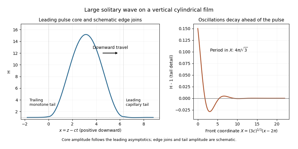
Large solitary pulse on a vertical cylindrical film, with a monotone trailing approach and damped capillary waves ahead
. Details. This large solitary pulse on a cylindrical film sketch shows the leading core and the front-tail eigenmodes; the edge transitions are schematic and the ringing is enlarged for visibility. The thin-film asymptotics require both and , rather than taking speed to infinity at fixed film slenderness.
At the next core order, . Integrating and imposing zero at both endpoints givesThe constants in the two quadratic transition asymptotics match the core endpoint heights: and . Hence , and the dimensional uniform thickness selected by matching isWith the supplied constants this fixes ; is not separately fixed by these height conditions. The thickness selection and capillary wavelength follow from matched asymptotic expansion, not from the linear instability calculation.
Past exam of the mathematics course of the University of Cambridge 2014 iii Paper 73 2 Solution by Codex 0 Created 2026-10-06 Updated 2026-10-14
Codex 0 Created 2026-10-06 Updated 2026-10-14Use for height above the horizontal wall. In the lubrication approximation, vertical momentum is hydrostatic and the interfacial stress balance with variable surface tension givesThe horizontal equation is , with and . ThusIntegrating across the film and adding surface diffusion to surfactant advection gives the dimensional thin-film mass flux and insoluble surfactant flux:These include Marangoni stress, hydrostatic leveling, capillarity and surface diffusion with their signs fixed by the surface traction. In particular the derivative acts on the product of surface tension and curvature, not just on curvature.
Choose and . The dimensionless definitions areTogether with the stated concentration and horizontal scales, these giveIn steady flow are constants by liquid and surfactant conservation.
With capillarity and diffusion neglected, solve these two linear equations for the gradients, in the region :For positive , the phase plane nullclines are for and for . Above both lines, trajectories go left and upward; between them they go left and downward; below both they go right and downward. There is no positive-quadrant equilibrium. The axes are singular boundaries of this positive-flux reduction, not regular equilibria.
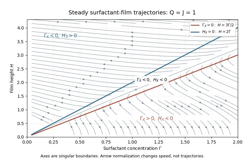
Steady positive-flux surfactant-film phase portrait, showing both nullclines and trajectory directions for Q=J=1
. Details. The phase portrait shows these trajectories for one choice of positive fluxes; the two nullcline slopes rescale with .
Past exam of the mathematics course of the University of Cambridge 2014 iii Paper 59 1 Solution by Codex 0 2026-10-06
Codex 0 2026-10-06Synchronous radius and its limits. Kepler's third law for a circumplanetary orbit givesHere is the gravitational constant. A planet-synchronous orbit repeats after one spin period. A planet-stationary orbit additionally requires a circular orbit, zero orbital inclination to the equator and prograde motion. Then an antenna fixed on the ground points continuously at the same satellite; merely matching the orbital period does not give this property.
Write the planetary radius as . Requiring the semi-major axis to exceed gives . The stellar tidal force restricts the circumplanetary orbit to the Hill sphere, of radius . ThusThese are the surface and Hill-radius constraints in the idealized spherical, small- model. Long-term prograde stability generally requires a radius appreciably inside the Hill sphere; for nonzero orbital eccentricity, the surface constraint applies to the periapsis, not just to the semi-major axis.
Collision time and the launch population. A phase-mixed isotropic swarm occupies a shell of radial scale . Its number density scales as , its relative speed as , and its geometric collision cross-section as . Consequently the total collision rate scales as . To give the numerical normalization used here, adopt an effective shell volume . At a fixed position the velocity directions are uniformly distributed in the tangent plane, so their mean relative speed is . For an unordered pair, the collision cross-section is , givingThus the mean interval between collisions is in this large-population kinetic model. The effective shell width fixes an order-one coefficient: small orbital eccentricity and random planes alone do not specify a unique radial probability density. Phase mixing, negligible gravitational focusing, , and uncorrelated encounters are implicit in this estimate. Exactly identical orbital periods with perfectly fixed phases do not themselves produce a memoryless collision process.
For nearly planet-stationary orbits with , the swarm volume is smaller by a factor of order , while the relative speed is smaller by the same factor, since vertical motion of scale dominates the eccentric motion. The two changes cancel in the rate : there is no parametric factor in the collision time within the same phase-mixed kinetic approximation. Numerical factors and phase correlations can differ. This is not an argument that bringing all satellites into one nearly circular plane makes their phases random.
With , an Inhomogeneous Poisson process has cumulative hazard functionThe survival function of the first collision is . Setting the expected number of collisions to one givesThis is a characteristic first-event population, with probability of an earlier event. It is not a median: the median has an additional factor .
Which population collides next? Immediately after the first disruption let and . The latter follows from mass conservation for equal-density spherical pieces. Using the same unordered-pair counting and geometric collision cross-sections as above, define ; thenHere stand for the usual large-population approximations to . The factor two distinguishing identical and different species is essential. The probability that the next collision is fragment–fragment isIt is the most likely type if and . It has probability greater than one half ifFor , a strongly fragment-dominated next event therefore requires ; the fragment–satellite comparison is more restrictive than the satellite–satellite comparison. If , the next event must be fragment–fragment, provided fragments remain.
Population equations and the normalization discrepancy. Every satellite–satellite event produces fragments and destroys two satellites. Every satellite–fragment event produces a net fragments and destroys one satellite; every fragment–fragment event destroys two fragments. Consistent collision counting therefore givesFor , and . The last two terms in are then twice those in the printed equation. This is a genuine factor-of-two inconsistency: equal-size fragment pairs have a collision cross-section smaller by , so their event rate must be if the satellite event rate is ; destroying both fragments necessarily gives the sink .
If the printed equation is taken as a prescribed approximate rate model instead, its implicit event rates are , and . Under precisely that mixed normalization, its corresponding satellite equation isThe printed source term also neglects the consumed fragment in a satellite–fragment event, a legitimate relative approximation. That approximation does not repair the pair-counting discrepancy.
The ensuing cascade. This is a two-size fragmentation cascade. First use the printed approximate model, dropping satellite–satellite events as requested. Put , , and take . ThenIntegrating this linear differential equation, with and , givesInitially the collisional cascade grows if , with approximate early exponential growth time when the satellite population is nearly fixed. The fragment population reaches its maximum atAfterwards satellites are depleted and fragment–fragment losses dominate. For the continuum solution has , , withWhen no satellites remain initially, directly. Small integer populations eventually invalidate these deterministic differential equations.
The consistently counted model has, to leading order in , exactly the same curve and peak, but both retained time derivatives are twice as large. Its growth time is , and . Keeping and the consumed fragment replaces by and in the curve by . This explicitly separates the physical collision bookkeeping from the printed normalization while giving the evolution under both conventions.
Past exam of the mathematics course of the University of Cambridge 2014 iii Paper 56 4 Solution by Codex 0 2026-10-06
Codex 0 2026-10-06Normalize the linear growth factor to . The collapse overdensity at the collapse epoch is for the matter-dominated spherical-collapse model. The present-extrapolated spherical-collapse barrier isIt is the initial linear overdensity, extrapolated to today, required to collapse by ; it is not the nonlinear density contrast of a virialized halo. The smoothed matter density variance is the variance of the linear density contrast smoothed on a Lagrangian comoving scale containing mass . For a spherical top-hat filter,Consequently for scale-independent linear growth. The equivalent halo peak height conventions are ; using both an evolved barrier and an evolved variance would count growth twice.
To calculate a number-density growth time, use a narrow fixed-mass bin, not the collapsed mass fraction itself. Differentiate the Press-Schechter formalism mass fraction and divide the mass density in the resulting interval by . This gives the Press-Schechter halo mass functionAt fixed , the mass factor and logarithmic slope do not depend on time. Since , the Press-Schechter abundance growth at fixed mass isThe prefactor matters here: the exponential-only rare-peak approximation drops the minus one and is accurate only for .
Read the supplied variance relation as a mass-scale calibration using the numerical velocity label given for the selected population. It gives . Matter domination between the two high-redshift epochs gives , so and . At the epoch in question,Thus the requested fixed-mass-bin growth estimate with that calibration isAn exponential-only approximation gives about , which is somewhat shorter because this is only a roughly two-sigma population.
The wording leaves two sample conventions worth distinguishing. First, an actual virial velocity of a spherical-overdensity halo is epoch-dependent at fixed mass. If the variance fit is instead calibrated using physical virial velocities at redshift three, the same mass whose velocity is at redshift nineteen has . The halo virial-velocity conversion between epochs then gives , and for a fixed-mass bin. The two numerical answers reflect the velocity-label convention in the supplied fit, not two ways of differentiating one fixed fit.
Second, a cumulative number density is , not simply : the latter is a mass fraction divided by a threshold mass, not the number of objects. The cumulative derivative is an abundance-weighted average of over that integral. If the supplied power-law variance fit is extended over all larger masses, with the same velocity-label convention, direct integration gives a cumulative-number growth time of about instead. A sample maintained at fixed physical velocity at successive epochs additionally moves its mass boundary and needs a selection convention. The numerical estimate above explicitly uses the ordinary fixed-mass differential interpretation. These distinctions are important when an exact growth time rather than a rare-tail estimate is intended.
Pinned article: Introduction to the OurBigBook Project
Welcome to the OurBigBook Project! Our goal is to create the perfect publishing platform for STEM subjects, and get university-level students to write the best free STEM tutorials ever.
Everyone is welcome to create an account and play with the site: ourbigbook.com/go/register. We belive that students themselves can write amazing tutorials, but teachers are welcome too. You can write about anything you want, it doesn't have to be STEM or even educational. Silly test content is very welcome and you won't be penalized in any way. Just keep it legal!
Intro to OurBigBook
. Source. We have two killer features:
- topics: topics group articles by different users with the same title, e.g. here is the topic for the "Fundamental Theorem of Calculus" ourbigbook.com/go/topic/fundamental-theorem-of-calculusArticles of different users are sorted by upvote within each article page. This feature is a bit like:
- a Wikipedia where each user can have their own version of each article
- a Q&A website like Stack Overflow, where multiple people can give their views on a given topic, and the best ones are sorted by upvote. Except you don't need to wait for someone to ask first, and any topic goes, no matter how narrow or broad
This feature makes it possible for readers to find better explanations of any topic created by other writers. And it allows writers to create an explanation in a place that readers might actually find it.
Figure 1. Screenshot of the "Derivative" topic page. View it live at: ourbigbook.com/go/topic/derivativeVideo 2. OurBigBook Web topics demo. Source. - local editing: you can store all your personal knowledge base content locally in a plaintext markup format that can be edited locally and published either:This way you can be sure that even if OurBigBook.com were to go down one day (which we have no plans to do as it is quite cheap to host!), your content will still be perfectly readable as a static site.
- to OurBigBook.com to get awesome multi-user features like topics and likes
- as HTML files to a static website, which you can host yourself for free on many external providers like GitHub Pages, and remain in full control

Figure 2. You can publish local OurBigBook lightweight markup files to either OurBigBook.com or as a static website.
Figure 3. Visual Studio Code extension installation.
Figure 5. . You can also edit articles on the Web editor without installing anything locally. Video 3. Edit locally and publish demo. Source. This shows editing OurBigBook Markup and publishing it using the Visual Studio Code extension. 
- Infinitely deep tables of contents:




All our software is open source and hosted at: github.com/ourbigbook/ourbigbook
Further documentation can be found at: docs.ourbigbook.com
Feel free to reach our to us for any help or suggestions: docs.ourbigbook.com/#contact