Topics (384k) Articles (398k) Users (410) Discussions (242) Comments (383) Files (13k) New article
For real , the Hermitian effective interaction is odd under time-reversal symmetry. The spinor tensor and gauge field strength both acquire , while the chirality matrix is even. Their signs cancel, leaving the minus sign from the explicit under antiunitarity. By the CPT theorem this is also CP violation. It is not a renormalizable tree-level Standard Model term, but a radiatively generated low-energy dipole is allowed because of the CP-violating phase in the CKM matrix.
A fermion bilinear transforming as a Lorentz four-vector. For a single Dirac field this is the Dirac current; distinct flavours can give a charged or flavour-changing current.
Strict monotonicity of Fermi gas entropy per particle by  Codex 0 Created 2026-10-05 Updated 2026-11-05
For density of states proportional to , , and positive temperature, set , , and . Differentiation and integration by parts giveThe inequality is strict Cauchy-Schwarz inequality, since is not constant under this positive weight. Thus fixed entropy per particle forces fixed . This is the injectivity step behind the adiabatic scaling of an ideal Fermi gas.
Adiabatic scaling of a Fermi gas with power-law density of states by Codex 0 Created 2026-10-05 Updated 2026-11-05
Codex 0 Created 2026-10-05 Updated 2026-11-05For density of states , , the grand canonical ensemble has . Strict monotonicity of Fermi gas entropy per particle makes constant at fixed entropy and particle number. Therefore and are constant along a reversible adiabatic process.
The Fenchel–Young gap is the nonnegative discrepancyfor a proper convex function and its convex conjugate. It can be . When is finite, it is the vertical distance between and its affine minorant . The Fenchel–Young gap vanishes exactly when , so it measures whether an input and a slope satisfy the subgradient relation.
For the convex quadratic function , completing the square givesAt and , the function value is and the tangent line has value , giving a Fenchel–Young gap of . In , the same calculation for gives and , half the squared Euclidean norm of the mismatch.
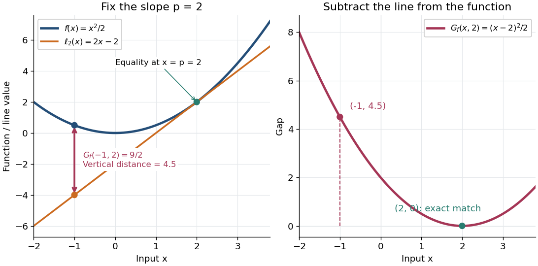
An exact optimization error certificate. Fix a slope with and minimize the linearly tilted objective function . By the definition of the convex conjugate, , soThis identity holds even when the infimum is not attained. Thus a computed finite Fenchel–Young gap is exactly the error in objective value for this minimization problem. For the convex quadratic function, implies . A general proper convex function need not convert a small gap into a small distance: the absolute value has zero gap at for every .
The Fenchel–Young gap also connects convex analysis to optimal transport. For a proper convex function , define Kantorovich potentials and . The half-squared Euclidean distance cost satisfies . For a transport plan with finite integrated cost and integrable Kantorovich potentials, integrating this identity gives the difference between transport cost and the potentials' bound. This is the same local subgradient mismatch summed over transported pairs.
For fixed positive integers and sufficiently large , the unique extremal graph forbidding vertex-disjoint copies of the complete graph is the join of graphs , up to isomorphic graphs. Each forbidden clique would require a distinct vertex of .
For a polynomial ring , a degree- polynomial polyvector field is an element of . Its product is the exterior product. Together with the Schouten-Nijenhuis bracket these spaces form a Gerstenhaber algebra.
The exterior product, also called the wedge product, combines oriented elements through the multiplicationFor two vectors, it is bilinear and alternating:These rules imply . They distinguish the exterior product from both the symmetric dot product and the unconstrained tensor product.[ref]
Linear Algebra Done Right by Sheldon Axler (4th edition). §9B, Definition 9.27 and Theorem 9.30, printed pp. 347–348: alternation and the sign of a swap
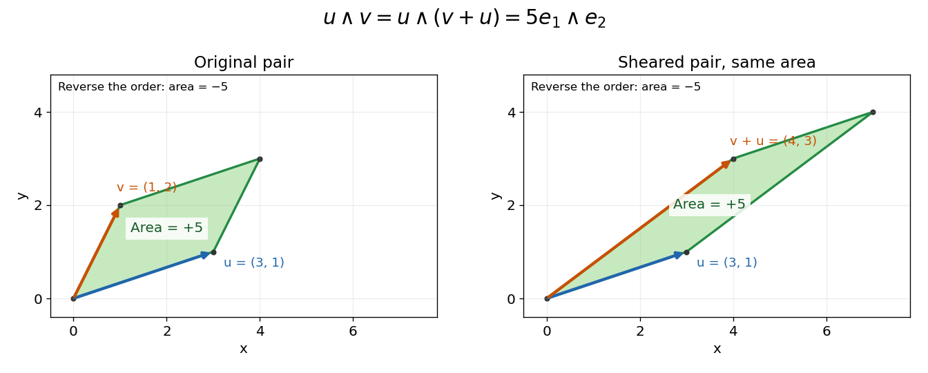
In an oriented orthonormal plane, write and . Expanding in its standard basis givesThe determinant is the signed area of the parallelogram formed by the two inputs. Its absolute value is the ordinary area. Reversing the input order reverses the sign; parallel inputs produce zero.
For the original example and ,Replacing by changes the shape but preserves the product: . Both parallelograms have the same oriented area element. If , the exterior product is zero, since .
The same rule adds directions in higher dimensions. With and the three-dimensional inputs under bivector,Its coefficient is the oriented volume of the three-dimensional parallelepiped. Repeating or linearly depending on earlier inputs collapses the volume, giving zero.
Partition the isomorphism classes of simple modules into two sets , with whenever lie in different sets. Every module of finite composition length then has a unique decomposition into its largest submodules whose Jordan–Hölder factors belong to the respective sets.
For a simple and a finite-length with factors in , induction through the long exact sequence of the Ext functor gives . Induct on the length of : take , split , and suppose . The quotient extension splits. The inverse image of its -summand complements in and has only factors in . Finally, Hom between modules with factors in different sets is zero, since any nonzero image would have a factor in both sets. Projecting any proposed submodule to the opposite summand therefore proves maximality and uniqueness.
Hyperbolic functions combine the exponential function to describe a hyperbola much as trigonometric functions describe a circle. Their two basic members are the hyperbolic cosine and hyperbolic sine, defined for every real number byTheir derivatives exchange the two functions:These formulas follow by applying differentiation to the exponential function definitions. [ref]
https://openstax.org/books/calculus-volume-2/pages/2-9-calculus-of-the-hyperbolic-functions. Gilbert Strang and Edwin Herman, OpenStax Calculus Volume 2, §2.9: hyperbolic definitions and derivatives
Adding and subtracting gives and . Multiplying these equalities proves the hyperbolic Pythagorean identity:Consequently the parametric equation traverses the entire right branch of the unit hyperbola , where . For example, gives , while gives approximately . Compare on the unit circle, where the squared coordinates add to one. The minus sign changes the geometry from a closed circle to an unbounded hyperbola.
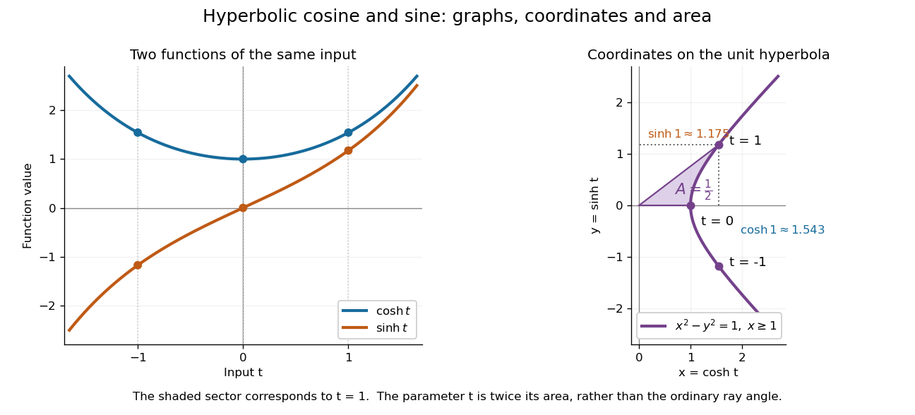
The other members are ratios and reciprocals: hyperbolic tangent is , hyperbolic cotangent is , and hyperbolic secant is ; denominators must be nonzero. The hyperbolic sine and hyperbolic cosine both solve the second-order linear differential equation . In fact has and , making this basis convenient for an initial value problem. Their geometry also makes hyperbolic substitution useful for integrals containing , and the hyperbolic cosine gives the physical catenary of a hanging chain.
For independent bond percolation on below the percolation critical probability, there are such that , uniformly in . This concerns the number of vertices in a percolation cluster, a stronger conclusion than decay of its radius alone.
Take a planet with opaque radius and an atmosphere of thickness , projected against a uniform stellar disc of radius . If the atmospheric annulus has one representative slant optical depth , its additional transit depth isThe general exoplanet transmission spectrum instead uses an integral over impact parameter ,The annulus model replaces this varying slant opacity by an effective constant. The atmospheric signal scales with optical depth when optically thin and saturates at the annular area when opaque.
Condensation followed by gravitational settling removes chemical elements from an atmospheric layer. The remaining gas may be in local chemical equilibrium with a depleted elemental inventory, while the column is not a closed equilibrium system.
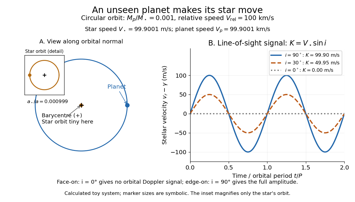
Doppler spectroscopy detects an exoplanet through the host star's changing Doppler shift. Both bodies orbit their shared astronomical barycenter: the star undergoes stellar reflex motion even when the exoplanet itself is unseen. Its velocity along the line of sight shifts its spectral lines; at speeds small compared with the speed of light, , with positive for recession. Repeated measurements can fit a Kepler orbit, rather than merely detect one shifted spectrum. Starspots and other changes in stellar spectral lines must be distinguished from actual orbital motion.
For one companion in an isolated two-body problem, the stellar radial-velocity semi-amplitude isHere is the gravitational constant, the orbital period, the orbital eccentricity, and the star and exoplanet masses. The orbital inclination is measured relative to the sky plane: is face-on and is an edge-on orbit. The exact binary mass function measured from the fitted orbit isWith known and , this is usually reported as . Taking gives the minimum companion mass; a smaller orbital inclination allows a larger mass. A detected exoplanet transit constrains close to for a compact planet orbiting well outside the star's surface, substantially resolving this ambiguity. Combining Doppler spectroscopy and exoplanet transit photometry then supplies a mass and radius for exoplanet interior studies.
For a computed circular example, let and choose a relative orbital speed : this is the speed of the planet relative to the star, not its speed about the astronomical barycenter. Conservation of momentum givesThe barycentric velocities point in opposite directions, so their speeds add to . Here and : at , at , and zero at . The star still orbits in the face-on case, but its orbital velocity has no line-of-sight component. The plotted circular signal is for a chosen phase origin and constant system velocity .
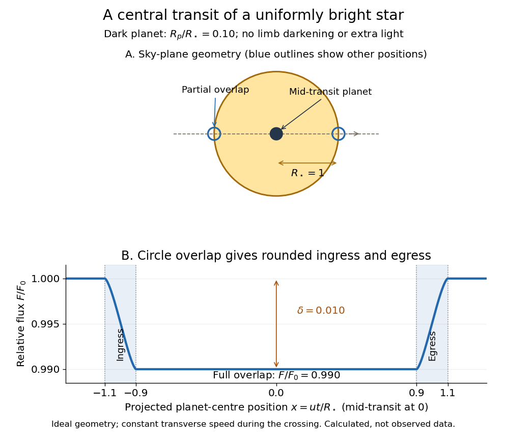
Exoplanet transit photometry measures the decrease in a star's observed radiative flux during an exoplanet transit. Define as the unobscured star's observed radiative flux and as the value at time . For a dark, opaque exoplanet crossing a uniformly bright circular stellar disc, a fully superimposed planetary disc blocks exactly the fractionHere and are the planet and star radii. This exoplanet transit depth determines a radius ratio, ; an absolute planet radius requires an independently estimated stellar radius. For , : a one-percent dip, with . Halving the radius ratio to reduces the exoplanet transit depth to , a quarter as much.
For the central exoplanet transit illustrated below, the transit impact parameter is . Write and let be the projected centre-to-centre separation in units of . The light curve is , where is the overlap area of circles of radii and . There is no overlap when ; the planetary disc is fully inside when , giving . Between those limits, the overlap area grows or shrinks continuously. Thus even a uniform star has curved ingress and egress, with a flat bottom only during full overlap. The illustration uses approximately constant transverse velocity over the short crossing, so with mid-transit at . Analytic models also handle limb darkening. [ref]
https://arxiv.org/abs/astro-ph/0210099. Mandel and Agol (2002)
.
The simple exoplanet transit depth formula assumes constant stellar brightness, no limb darkening or starspots, negligible light from the exoplanet, and no transit dilution by other light. It describes full overlap in a non-grazing exoplanet transit, requiring for a full-overlap interval. A grazing exoplanet transit never hides the whole planetary disc against the star, and limb darkening weights different blocked areas differently. Repeating dips are valuable evidence, but eclipsing binary stars and starspots can imitate parts of the signal, so confirmation and joint modelling matter.
The Very Large Telescope is an observatory array at Paranal with four -metre Unit Telescopes and four movable -metre Auxiliary Telescopes. The Unit Telescopes can observe independently; selected beams can also be combined in an astronomical interferometer. Combining beams coherently changes the angular information available and requires an appropriate observing instrument.[ref]
Very Large Telescope overview by European Southern Observatory. Overview: telescope diameters, independent operation, and interferometric combination
For exoplanets, adaptive optics helps concentrate light for exoplanet direct imaging, while instruments such as CRIRES resolve molecular spectral lines. Spatial separation and Doppler shift provide complementary ways to distinguish a faint planet from its host star. The capability belongs to the telescope-plus-instrument combination, rather than to aperture size alone.
An exoplanet thermal phase curve measures the change in planetary infrared brightness through the orbit, after modelling the host star's contribution. Around exoplanet secondary eclipse the visible hemisphere is mostly dayside; around primary exoplanet transit it is mostly nightside. The amplitude therefore constrains the longitudinal thermal contrast, while an offset maximum indicates an asymmetric brightness distribution.
Spitzer Space Telescope observations of HD 189733 b demonstrated that this technique could constrain day-night heat redistribution and a displaced bright region even without resolving the planetary disc.[ref]
A map of the day-night contrast of the extrasolar planet HD 189733b by Heather A. Knutson and others. Abstract: half-orbit brightness variation and offset peak
A phase curve averages light over a visible hemisphere. Its map is therefore model-dependent, and brightness temperatures in one band need not describe all atmospheric pressures.The atmospheric advection time over length at wind speed is . Day-night heat redistribution tends to be efficient when this time and the relevant wave-adjustment time are shorter than the radiative relaxation time in a planetary atmosphere.
A column near pressure contains mass per area of order . Linearizing its blackbody cooling around temperature gives the estimatewhere is specific heat capacity at constant pressure. This estimate omits details of wavelength-dependent radiative transfer, but captures faster relaxation in hotter and lower-pressure atmospheric layers.
For an integer-valued underlying with European call option prices , the second strike difference equals . It is the discrete counterpart of recovering a payoff probability distribution from strike derivatives.
Pinned article: Introduction to the OurBigBook Project
Welcome to the OurBigBook Project! Our goal is to create the perfect publishing platform for STEM subjects, and get university-level students to write the best free STEM tutorials ever.
Everyone is welcome to create an account and play with the site: ourbigbook.com/go/register. We belive that students themselves can write amazing tutorials, but teachers are welcome too. You can write about anything you want, it doesn't have to be STEM or even educational. Silly test content is very welcome and you won't be penalized in any way. Just keep it legal!
Intro to OurBigBook
. Source. We have two killer features:
- topics: topics group articles by different users with the same title, e.g. here is the topic for the "Fundamental Theorem of Calculus" ourbigbook.com/go/topic/fundamental-theorem-of-calculusArticles of different users are sorted by upvote within each article page. This feature is a bit like:
- a Wikipedia where each user can have their own version of each article
- a Q&A website like Stack Overflow, where multiple people can give their views on a given topic, and the best ones are sorted by upvote. Except you don't need to wait for someone to ask first, and any topic goes, no matter how narrow or broad
This feature makes it possible for readers to find better explanations of any topic created by other writers. And it allows writers to create an explanation in a place that readers might actually find it.
Figure 1. Screenshot of the "Derivative" topic page. View it live at: ourbigbook.com/go/topic/derivativeVideo 2. OurBigBook Web topics demo. Source. - local editing: you can store all your personal knowledge base content locally in a plaintext markup format that can be edited locally and published either:This way you can be sure that even if OurBigBook.com were to go down one day (which we have no plans to do as it is quite cheap to host!), your content will still be perfectly readable as a static site.
- to OurBigBook.com to get awesome multi-user features like topics and likes
- as HTML files to a static website, which you can host yourself for free on many external providers like GitHub Pages, and remain in full control

Figure 2. You can publish local OurBigBook lightweight markup files to either OurBigBook.com or as a static website.
Figure 3. Visual Studio Code extension installation.
Figure 5. . You can also edit articles on the Web editor without installing anything locally. Video 3. Edit locally and publish demo. Source. This shows editing OurBigBook Markup and publishing it using the Visual Studio Code extension. 
- Infinitely deep tables of contents:




All our software is open source and hosted at: github.com/ourbigbook/ourbigbook
Further documentation can be found at: docs.ourbigbook.com
Feel free to reach our to us for any help or suggestions: docs.ourbigbook.com/#contact