Topics (384k) Articles (398k) Users (410) Discussions (242) Comments (383) Files (13k) New article
Past exam of the mathematics course of the University of Cambridge 2010 iii Paper 15 1 a Solution by  Codex 0 Created 2026-10-03 Updated 2026-10-14
An integral curve of a vector field through is a smooth curve , on an interval containing zero, satisfying and . The local flow is the smoothly varying family of these integral curves of a vector field:Here is an open neighborhood of ; for the maximal local flow, its fibre over is the maximal existence interval of . Local existence, uniqueness and smooth dependence for a smooth ordinary differential equation give this family. Uniqueness also gives whenever the relevant curves and compositions are defined, and on their common domains.
Past exam of the mathematics course of the University of Cambridge 2010 iii Paper 14 5 b Solution by Codex 0 Created 2026-10-03 Updated 2026-10-14
Codex 0 Created 2026-10-03 Updated 2026-10-14We use the following precise degree-zero/one kernel of the magnetic X-ray transform in degrees zero and one theorem, as permitted here: for a smooth Anosov magnetic flow on a closed oriented surface, ifwith a smooth base function and a smooth one-form, then and is exact. Exact one-forms give the converse, because . No assumption of pointwise negative Gaussian curvature is needed for this theorem. We now derive the contact obstruction from it rather than assume the desired rigidity conclusion.
Use the usual connected-surface convention. Since , the top-degree de Rham cohomology class of vanishes: integration identifies with . Choose a smooth one-form on satisfying , and setThe structure equations and the previous volume calculation giveThis primitive exists because of the zero-flux hypothesis, and need not itself be contact.
A useful elementary fact is that every smooth invariant function of an Anosov flow is constant on a connected manifold. If , then , and boundedness of with exponential contraction makes this zero as . Negative time does the same for an unstable vector. Also . The Anosov splitting spans the tangent space, so . This avoids any extra ergodicity assumption.
Suppose a smooth contact form is preserved. Invariance and contraction imply in the limit; negative time gives the same on unstable vectors. Thus annihilates both transverse bundles. Its value cannot vanish anywhere, since otherwise would be zero at that point, contradicting the contact condition. It is a smooth invariant function and therefore a nonzero constant. Divide by that constant to arrange .
The Cartan formula for the Lie derivative now gives . In dimension three, all two-forms annihilating are scalar multiples of , soThe scalar is smooth and nowhere zero by the contact condition. Both sides without are flow-invariant; hence and the preceding Anosov argument makes constant. It follows thatis a closed differential one-form.
We require the Liouville mean of such a closed differential form, and derive it explicitly. Let be fibre rotation and average over . Since , the Cartan formula for the Lie derivative givesConsequently its rotational average differs from by an exact form. For a closed rotationally invariant one-form , the identity makes its vertical value a constant . Subtracting leaves a rotationally invariant horizontal form, which descends to a base form . We have therefore proved the averaging closed one-forms on a surface unit tangent bundle decompositionThe last relation follows from closedness and .
Evaluation at gives . The average of the linear expression around each unit circle is zero. The second term has total integral . Finally by volume preservation and Stokes theorem. Thusfor every closed differential one-form in this zero-flux system. Apply this to : the directional average of also vanishes, so its integral is . Positivity of the volume forces . Hence and is closed.
Using its proved decomposition and , we obtainThe stated magnetic transform kernel theorem gives and exactness of , hence . If , then and , so . If , the equation already gives . Necessity is proved.
Conversely, if , then . The canonical form is contact because never vanishes, andThus the flow preserves , provingIf disconnected surfaces are admitted, the flux condition must hold on each component for the exactness step; a single cancelling total flux does not imply componentwise exactness. The result above uses the standard connected interpretation of a surface.
Past exam of the mathematics course of the University of Cambridge 2010 iii Paper 14 5 a Solution by Codex 0 Created 2026-10-03 Updated 2026-10-14
Codex 0 Created 2026-10-03 Updated 2026-10-14The forcing is perpendicular to velocity, soStarting at unit speed therefore keeps the motion in . The horizontal part is the geodesic transport , while the acceleration rotates the unit velocity at angular speed . Thus the magnetic flow generator is .
For the canonical coframe of a surface unit tangent bundle, set . Its interior product of a differential form with the two relevant fields isThe structure equations giveThe Cartan formula for the Lie derivative consequently gives . For the variable vertical coefficient, use the full product rule:Indeed is pulled back from the base, so and has only components. HenceThe Liouville volume of a surface geodesic flow is therefore preserved by this magnetic modification for every smooth , without requiring the Anosov property.
Past exam of the mathematics course of the University of Cambridge 2010 iii Paper 14 4 b Solution by Codex 0 Created 2026-10-03 Updated 2026-10-14
Codex 0 Created 2026-10-03 Updated 2026-10-14Use the canonical coframe of a surface unit tangent bundle and its dual . In constant curvature , the decaying normal Jacobi fields have data , so the stable line is generated by . The weak stable bundle is thereforeIt is annihilated by the nonvanishing form . The structure equations now giveThus the auxiliary form in the Godbillon-Vey invariant can be taken as . In the natural orientation given by the oriented base and positive fibre rotation, put . ThenThis sign is important: in these conventions the contact three-form is the negative of the positive Liouville volume of a surface geodesic flow.
Integration around each circle fibre gives , while . Hence . The Gauss-Bonnet theorem and give . ConsequentlyFor genus , this is in the stated orientation. The opposite orientation of reverses the sign.
Past exam of the mathematics course of the University of Cambridge 2010 iii Paper 14 4 a Solution by Codex 0 Created 2026-10-03 Updated 2026-10-14
Codex 0 Created 2026-10-03 Updated 2026-10-14A coorientation gives a globally nonvanishing one-form with . For tangent fields in the integrable distribution,since integrability makes their bracket tangent to . Thus . Choose a transverse field with . The one-form then satisfies , as is checked on and .
The Godbillon-Vey invariant in the unnormalized convention isThe three-form is continuous at the specified regularity, so its integral is defined. We prove independence of both choices by producing exact differences with primitives, allowing ordinary Stokes theorem.
First, for a fixed , another admissible auxiliary form has the form . From and , one gets . Expanding the two three-forms, using this relation and , givesIts integral on the closed manifold vanishes.
Next any other defining form is with nowhere zero. Let . Thenso one may use . Its three-form differs byAgain the difference integrates to zero; any subsequent auxiliary choice is handled by the first calculation. This includes reversing the chosen coorientation, since can be negative. Thus the invariant, and the corresponding de Rham cohomology class, depends only on the oriented manifold and the foliation defined by . Reversing the orientation of , unlike reversing the coorientation of , changes the sign of its numerical value.
Past exam of the mathematics course of the University of Cambridge 2010 iii Paper 14 3 c Solution by Codex 0 Created 2026-10-03 Updated 2026-10-14
Codex 0 Created 2026-10-03 Updated 2026-10-14Full equality of the Riemannian metrics at the boundary identifies their boundary unit bundles, outward normals and induced boundary Riemannian metrics. We show directly that the common boundary distance function determines both endpoint directions.
For distinct boundary points , let be the unique joining unit-speed geodesic, with initial velocity and final velocity . The first variation of its length gives, for and ,Indeed, integration by parts in the length variation leaves just the endpoint terms, because the interior term contains . The Riemannian metric is simple, so the off-diagonal endpoint dependence is smooth and these derivatives are valid.
Thus the tangential components are and . Unit speed and the incoming/outgoing signs supply the missing normal components:All quantities on the right use only boundary distance and the common boundary Riemannian metric. Every strictly incoming vector for has some exit point ; the geodesic joining the same pair for has exactly the same reconstructed initial and final vectors. Hence both geodesic scattering relations give the same exit for that input. Tangential vectors are fixed, and the outgoing extensions agree as inverses. ThereforeIn fact their exit times also agree, since each is .
Past exam of the mathematics course of the University of Cambridge 2010 iii Paper 14 3 b Solution by Codex 0 Created 2026-10-03 Updated 2026-10-14
Codex 0 Created 2026-10-03 Updated 2026-10-14First the common boundary distance function determines the induced tangential Riemannian metric. For a boundary curve with and , the local first-order distance expansion givesFor clarity, the upper bound follows from the length of the boundary curve. In a small coordinate neighbourhood the Riemannian metric is arbitrarily close to its value at , so the length of any sufficiently short joining path is bounded below by that constant-metric displacement norm with an arbitrarily small relative error. A minimizing short path cannot leave that neighbourhood. These two bounds prove the limit. Equality of the boundary distance functions then gives . The polarization identity yieldsThis alone fixes no choice of normal coordinates, so a boundary-fixing gauge is needed to compare the full tangent-space Riemannian metrics.
Let be the inward unit normals and letbe sufficiently small boundary normal coordinates. Their pullbacks have the form , with . On a collar define . It fixes the boundary, has for tangential , and sends to . For tangent-space vectors and at the boundary, therefore,This proves the desired full Riemannian metric equality locally at the boundary.
We also justify extending this local identification to a global diffeomorphism. Interpolate the positive Riemannian metrics by , for . Let be their inward unit-normal exponential collars. Compactness of the boundary and parameter interval gives a common small collar width for all . The intermediate Riemannian metrics need not be simple; only these local collars are used.
On the image of , define the time-dependent vector fieldwhere is one near zero and vanishes before the outer edge of the collar; extend by zero elsewhere. This is a smooth vector field on , vanishing at the boundary because . Its time-dependent flow is a global diffeomorphism fixing the boundary. For every sufficiently small fixed , the curve solves its equation, since . Uniqueness gives . Consequently agrees near the boundary with . Taking proves
Past exam of the mathematics course of the University of Cambridge 2010 iii Paper 14 3 a Solution by Codex 0 Created 2026-10-03 Updated 2026-10-14
Codex 0 Created 2026-10-03 Updated 2026-10-14A simple Riemannian manifold has strictly convex boundary and a unique geodesic between each pair of points, smoothly dependent on its endpoints; there are no conjugate points and no trapped geodesics. Let denote the outward unit normal. For a boundary unit vector with , follow its unit-speed geodesic until the next boundary intersection at time . Its geodesic scattering relation isThus it maps incoming boundary unit vectors to outgoing ones, recording both exit point and direction.
If the scattering relation is defined on the full boundary unit bundle, extend it on outgoing vectors by following the same oriented geodesic backwards to its previous boundary intersection, and fix tangential vectors. This extension is an involution, because the second application follows the same segment back to its starting point with the same velocity. The exit time is not a component of the scattering relation itself; together with it one obtains lens data. For a simple Riemannian metric, is the boundary distance between the endpoints of the segment.
Past exam of the mathematics course of the University of Cambridge 2010 iii Paper 14 2 c Solution by Codex 0 Created 2026-10-03 Updated 2026-10-14
Codex 0 Created 2026-10-03 Updated 2026-10-14Use the given Pestov identity for a geodesic flow for the function constructed above. Since , its left side is . Moving this to the right givesAll terms are nonnegative, and is uniformly positive by compactness. The smooth derivatives therefore vanish pointwise:Since span the tangent bundle, is constant, component by component if necessary.
On each circle fibre, is the elementary periodic differential equation . Its solutions areThe first harmonics transform as a covector when the local oriented orthonormal frame changes. Their coefficients are smooth, either directly from the smooth fibre equation or from their sine/cosine integral formulas. Thus they define a smooth one-form on with .
Along a geodesic, the velocity is parallel, so differentiating givesSet . ThenEquality initially holds on unit vectors, then on every vector by homogeneity. The polarization identity yields the tensor identityThis proves that is a potential symmetric 2-tensor, with the precise factor of two in the requested convention.
Past exam of the mathematics course of the University of Cambridge 2010 iii Paper 14 2 b Solution by Codex 0 Created 2026-10-03 Updated 2026-11-05
Codex 0 Created 2026-10-03 Updated 2026-11-05The geodesic flow of a closed negatively curved surface is a topologically transitive Anosov flow. In particular, its Jacobi-field hyperbolicity and the usual negative-curvature transitivity theorem allow the smooth Livšic theorem to be applied. Set . The given closed-geodesic integrals are exactly its periodic-orbit obstructions on . Therefore
We make the differential operators and signs explicit. On the unit tangent bundle, let generate positive fibre rotation, be the geodesic vector field and . For the canonical coframe of a surface unit tangent bundle, writeand let be the Levi-Civita connection form with . This uses for a one-form, keeping for the given tensor. The dual frame is , and the structure equations areThese follow by writing the two horizontal forms as a rotated local orthonormal coframe and , with its connection 1-form. Equivalently, differentiating the sine and cosine components of twice in the fibre angle givesThe curvature equation also gives . The Liouville volume of a surface geodesic flow will be taken positive in the base/positive-fibre orientation, namely .
The Lie bracket of vector fields identities give an operator identity that supplies the required equation. First,Using and , differentiate this expression once more to obtainFor and , the first term vanishes by the explicit fibre calculation. Hence
Past exam of the mathematics course of the University of Cambridge 2010 iii Paper 14 2 a Solution by Codex 0 Created 2026-10-03 Updated 2026-11-05
Codex 0 Created 2026-10-03 Updated 2026-11-05The Livšic theorem for a topologically transitive Anosov flow says that a Hölder function satisfies the periodic-orbit obstructionif and only if there is a Hölder function satisfying the flow coboundary identityThe solution is differentiable along orbits and in that sense. For a smooth flow and smooth , the smooth regularity version gives , so holds smoothly. The solution is unique up to an additive constant: the difference of two solutions is invariant and must be constant on a dense orbit and then everywhere by continuity. Necessity of the periodic obstruction follows immediately by taking in the displayed identity.
Past exam of the mathematics course of the University of Cambridge 2010 iii Paper 14 1 b Solution by Codex 0 Created 2026-10-03 Updated 2026-10-14
Codex 0 Created 2026-10-03 Updated 2026-10-14Put and denote the flow generated by by . It follows the same oriented orbits as , with the clock determined implicitly byBecause is positive on a compact manifold, and for . Negative times obey the corresponding absolute-value comparison. This makes it possible to transfer exponential estimates once the correct transverse graphs are found.
For defineThe integrand is bounded by a constant times , since is bounded and is stable. The integral converges uniformly on bounded bundle vectors, so it is continuous and linear in . Consider the graphWe verify its invariance and contraction directly; the old Anosov stable bundle need not itself remain invariant under a positive time change of a smooth flow.
For a fixed old time , setDifferentiation gives and . Differentiating the implicit clock at fixed , then differentiating , therefore yields for For this becomesThe tail coefficient equals by the flow composition law, proving graph invariance. Both the first term and the tail have norm at most . Projection onto in the original splitting is uniformly bounded, hence . The clock comparison now givesFor the Anosov unstable bundle, use the convergent past integralThe same differentiation formula gives the tail for , proving invariance and exponential contraction in negative new time.
Finally, these two graphs and form a direct splitting. Projecting onto identifies the graphs with the old complementary stable and unstable subspaces, so they intersect neither each other nor the centre. We have established the continuous invariant splitting and both uniform estimates, and therefore the flow of is Anosov.
Past exam of the mathematics course of the University of Cambridge 2010 iii Paper 14 1 a Solution by Codex 0 Created 2026-10-03 Updated 2026-10-14
Codex 0 Created 2026-10-03 Updated 2026-10-14For a nonsingular smooth flow generated by on a closed manifold, the Anosov flow condition is a continuous -invariant splittingand constants such that, for all ,The norm can come from any auxiliary Riemannian metric; compactness makes the resulting definitions equivalent. The centre direction is the flow direction, with nowhere zero.
One construction is a suspension flow. The hyperbolic toral automorphism of defined byhas eigenvalues , with . Form the closed three-dimensional mapping torus and move in the second coordinate at unit speed. Each crossing of the section applies . The two one-dimensional eigenspaces give invariant transverse bundles, and after crossings their derivatives multiply by and . The difference between and elapsed time is bounded, so any smooth Riemannian metric gives the required uniform exponential estimates. The vertical direction supplies the centre line.
A different construction is the geodesic flow on the unit tangent bundle of a closed oriented hyperbolic surface. This bundle is a closed three-manifold. In curvature , a normal Jacobi field along a unit-speed geodesic satisfies . The initial data give , while give . The linearized geodesic flow transports these initial data as , so they give one stable and one unstable direction with precisely those exponential rates. The remaining tangent direction is the geodesic vector field. Thus this also constructs an Anosov flow, using geometric rather than return-map hyperbolicity.
Past exam of the mathematics course of the University of Cambridge 2010 iii Paper 12 4 ii Solution by Codex 0 Created 2026-10-03 Updated 2026-10-14
Codex 0 Created 2026-10-03 Updated 2026-10-14Write , an integer under the stated divisibility assumption. The degree relation gives . Take the disjoint union of graphs of copies of the complete bipartite graph , placing its -vertex part in and its -vertex part in . The total part sizes are then and . Each left vertex has vertex degree , and each right vertex has vertex degree , so the graph has exactly the required biregular graph parameters.
An independent set in one component can be any subset of its left part or any subset of its right part. It cannot contain a vertex from both parts, because all cross-pairs are edges. The two families share only the empty set, so the component has independent sets. Choices in different connected components of a graph are independent combinatorial choices, and their counts multiply. HenceThis attains equality in part (i). It also explains the entropy weight there: the empty selected left neighbourhood permits all subsets of the opposite part.
Past exam of the mathematics course of the University of Cambridge 2010 iii Paper 12 4 i Solution by Codex 0 Created 2026-10-03 Updated 2026-10-14
Codex 0 Created 2026-10-03 Updated 2026-10-14Let be the number of independent sets of the biregular graph . Choose one such set uniformly and write . All information entropies below use logarithms to base two, soWe will prove .
We state and justify the entropy facts used. For a finite-valued random variable , with . Its conditional entropy is the mean of this quantity over the conditioning variable. Factoring the joint probabilities proves the chain rule for information entropy, . Conditioning reduces entropy: . To see this, condition on and use concavity of to compare the mixture of the conditional distributions given with their mean entropy.
The precise Shearer inequality needed here is: if subsets of the indices of a finite random vector cover every index at least times, then . To prove it, order the indices. The chain rule for information entropy expandsThe inequality is conditioning reduces entropy. Summing over counts each nonnegative conditional term at least times and proves the assertion.
For every , its vertex neighbourhood has vertices. Every lies in exactly of these neighbourhoods. Hence Shearer inequality givesLet , the probability that no neighbour of is selected. Conditional on a particular selected subset of , a vertex with a selected neighbour is forbidden, and all other vertices of are available. Because there are no edges within , every subset of the available vertices is a valid completion. Uniform choice of makes these completions equally likely. The available coordinates are therefore independent fair binary choices, each of entropy one, and the forbidden coordinates are zero. Averaging their number givesBy the chain rule for information entropy,It remains to bound each bracket. Let , a binary vector of length , with distribution on , and put . Assign weight to the all-zero vector and weight to every nonzero vector. ThenThe first inequality is Jensen's inequality for the concave logarithm; the weights sum to . This explicitly handles zero probabilities and does not assume the neighbourhood indicators are independent.
There are right vertices, so combining the bounds and using givesExponentiating proves the required independent-set bound for biregular graphs. The proof uses both degree constraints: supplies the neighbourhood-cover multiplicity and the conditional-completion weight, while determines the number of neighbourhood patterns.
Past exam of the mathematics course of the University of Cambridge 2010 iii Paper 12 3 iii Solution by Codex 0 Created 2026-10-03 Updated 2026-10-14
Codex 0 Created 2026-10-03 Updated 2026-10-14The precise external concentration result we use is Talagrand's convex distance inequality: for a finite product of independent standard probability spaces, a measurable event of positive probability, and ,Our coordinates are the independent uniformly sampled points of the triangle, so the hypothesis holds. Part (ii) therefore gives, for integers ,Indeed every configuration in the first event has at least the distance from part (ii) to the second event. If one event is empty, the displayed product bound is automatic. This is the only use of the product-space theorem; the geometric separation was proved directly in part (ii). A precise source for that theorem is Section 4.1 of Talagrand's original product-space concentration paper.
Choose an integer median , so and . First set , in the product bound, and then set , . For positive integers this yields the convex-chain median concentration estimatesThe lower event is empty if in our sampling model; the upper event is empty if . Thus the stated bounds remain valid for all positive integers . Also for .
By part (i), with . Let , take , and use the deterministic interval . Its length is exactly . As and are integers, falling outside this interval implies one of the two tail events with . ThereforeFor positive ,Since and , this exponent is at leastConsequentlyThus lies with high probability in the required interval. This proof works for every , including growth faster than ; no extra restriction on is needed. The scale comes from the square root of the certificate size at the median.
Past exam of the mathematics course of the University of Cambridge 2010 iii Paper 12 3 ii Solution by Codex 0 Created 2026-10-03 Updated 2026-10-14
Codex 0 Created 2026-10-03 Updated 2026-10-14We use the directed set version of the Talagrand convex distance:Here a coordinate is an entire sampled point, so means the two planar points differ. This is the distance from the upper event to the lower event ; its order is relevant because the convex distance need not be symmetric.
Fix and choose exactly indices whose points form a convex chain with the endpoints. Such a choice exists even if , by taking a subchain. It is a certificate of the certifiable function . For any , let . The unchanged selected points remain a convex chain in configuration , soChoose the nonnegative weights for and zero otherwise. They have squared sum one, and for every ,Taking the infimum over , then the supremum over weights, and finally the infimum over provesThis proof also works for if zero-length chains are admitted, and gives the usual infinite separation when one of the events is empty. For the uniform sampling model, almost surely when .
Past exam of the mathematics course of the University of Cambridge 2010 iii Paper 12 3 i Solution by Codex 0 Created 2026-10-03 Updated 2026-10-14
Codex 0 Created 2026-10-03 Updated 2026-10-14Take the sampled points to be independent with the uniform distribution on . Its area is , so its probability density is two. With probability one there are no coincidences, equal relevant coordinates or collinear triples. We give an exact first moment method argument; no tangent construction is needed.
First count the probability that labelled points, together with the endpoints, form a convex chain. In their order along the lower boundary, write their coordinates as , , and put , . They necessarily satisfyIndeed the lower boundary of the convex polygon is the graph of a convex piecewise linear function. Its segment slopes strictly increase; the first is positive because the first point lies above the axis, making all later slopes positive too.
Set and for . Both spacing vectors lie in the open probability simplex, with . The coordinate-monotone region has volume . The change to the first spacings in each vector has Jacobian one, and each simplex has uniform volume measure. Simultaneous permutation of all pairs preserves this product volume measure. Except on a null set of ties, the ratios therefore have all possible orders with equal volume.
Strict increase of these ratios is exactly the convex chain condition. It also puts the intermediate points below the diagonal: the weighted mean of all slopes is , and each proper initial weighted mean is strictly smaller than one, so for . Thus it suffices to impose the slope order on the whole coordinate-monotone region; no additional triangle restriction is needed.
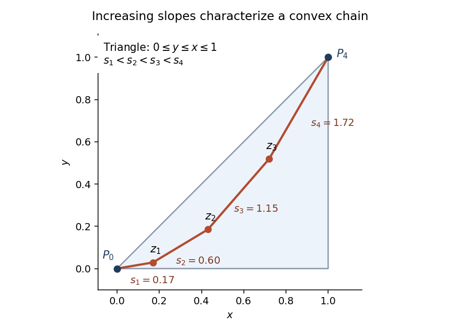
The volume for one specified label order is consequently . There are disjoint orders of the labels, and the joint uniform-triangle density is . Hence the convex-chain probability in a triangle isFor example and .
Let count the -element subsets of the sampled points that are convex chains. By linearity of expectation, . If , an optimal chain contains a -vertex subchain, since removing vertices from a convex polygon preserves convex position of the remaining vertices. Therefore, by the first moment method,We used , , and , the last following from .
Take . If , the last bound is at most ; if , the event is empty. Every integer median must then satisfy , and thereforeThe hint's curve is a parabola, not a hyperbola. The exact counting argument above proves the upper bound directly. The same chain probability is recorded in Ambrus and Bárány's analysis of longest convex chains.
Past exam of the mathematics course of the University of Cambridge 2010 iii Paper 12 2 ii Solution by Codex 0 Created 2026-10-03 Updated 2026-10-14
Codex 0 Created 2026-10-03 Updated 2026-10-14Put , and define . The triangle inequality shows that is Lipschitz continuous with Lipschitz constant one. It vanishes on , and on . Let for a uniform permutation.
If , apply the lower-tail bound proved in part (i):If , apply its upper-tail bound:For the desired inequality is simply . Hence in all casesThis uses only the precise one-sided concentration inequality from part (i) and the Hamming distance triangle inequality. The normalization of the distance matters: it counts mismatching coordinates, rather than dividing their number by .
Past exam of the mathematics course of the University of Cambridge 2010 iii Paper 12 2 i Solution by Codex 0 Created 2026-10-03 Updated 2026-10-14
Codex 0 Created 2026-10-03 Updated 2026-10-14Use the uniform probability measure on the symmetric group and the unnormalized Hamming distanceLet have Lipschitz constant for this distance. We will prove the one-sided concentration inequalitiesConsequently for . A zero Lipschitz constant makes constant, so that case is immediate.
Let be a uniform permutation, reveal successively, and define the Doob exposure martingaleFix the first images. For an available value , let be the conditional mean when . Given two available values , left-composition with the transposition exchanging is a bijection from completions with next image to completions with next image . It fixes the previously exposed images and changes exactly two coordinates of each complete permutation. Since conditional completions are uniform, averaging the Lipschitz condition over this pairing gives .
Thus, conditionally on the first images, has mean zero and takes values in an interval of length at most . We need the range-length version of the Hoeffding lemma: if a real random variable has mean zero and lies in an interval of length , thenHere is a proof. For , differentiation gives under the exponentially tilted probability distribution. Any distribution on an interval of length has variance at most , because its squared distance from the interval midpoint is at most . Since , integrating this second-derivative bound gives the lemma for both signs of . The same argument holds for every conditional distribution.
Apply it conditionally to each martingale difference and use the tower property of conditional expectation repeatedly:The exponential Markov bound now gives, for ,Choose to obtain the upper tail in the box, and apply the argument to for the lower tail. This proves concentration of Lipschitz functions on the symmetric group. Using only the bound in the absolute-increment Azuma-Hoeffding inequality would lose a factor four in the exponent; the conditional range length is what yields the constant needed in part (ii).
Pinned article: Introduction to the OurBigBook Project
Welcome to the OurBigBook Project! Our goal is to create the perfect publishing platform for STEM subjects, and get university-level students to write the best free STEM tutorials ever.
Everyone is welcome to create an account and play with the site: ourbigbook.com/go/register. We belive that students themselves can write amazing tutorials, but teachers are welcome too. You can write about anything you want, it doesn't have to be STEM or even educational. Silly test content is very welcome and you won't be penalized in any way. Just keep it legal!
Intro to OurBigBook
. Source. We have two killer features:
- topics: topics group articles by different users with the same title, e.g. here is the topic for the "Fundamental Theorem of Calculus" ourbigbook.com/go/topic/fundamental-theorem-of-calculusArticles of different users are sorted by upvote within each article page. This feature is a bit like:
- a Wikipedia where each user can have their own version of each article
- a Q&A website like Stack Overflow, where multiple people can give their views on a given topic, and the best ones are sorted by upvote. Except you don't need to wait for someone to ask first, and any topic goes, no matter how narrow or broad
This feature makes it possible for readers to find better explanations of any topic created by other writers. And it allows writers to create an explanation in a place that readers might actually find it.
Figure 1. Screenshot of the "Derivative" topic page. View it live at: ourbigbook.com/go/topic/derivativeVideo 2. OurBigBook Web topics demo. Source. - local editing: you can store all your personal knowledge base content locally in a plaintext markup format that can be edited locally and published either:This way you can be sure that even if OurBigBook.com were to go down one day (which we have no plans to do as it is quite cheap to host!), your content will still be perfectly readable as a static site.
- to OurBigBook.com to get awesome multi-user features like topics and likes
- as HTML files to a static website, which you can host yourself for free on many external providers like GitHub Pages, and remain in full control

Figure 2. You can publish local OurBigBook lightweight markup files to either OurBigBook.com or as a static website.
Figure 3. Visual Studio Code extension installation.
Figure 5. . You can also edit articles on the Web editor without installing anything locally. Video 3. Edit locally and publish demo. Source. This shows editing OurBigBook Markup and publishing it using the Visual Studio Code extension. 
- Infinitely deep tables of contents:



All our software is open source and hosted at: github.com/ourbigbook/ourbigbook
Further documentation can be found at: docs.ourbigbook.com
Feel free to reach our to us for any help or suggestions: docs.ourbigbook.com/#contact