
Past exam of the mathematics course of the University of Cambridge 2009 ib Paper 2 10G Solution Created 2026-09-24 Updated 2026-10-14
The ascending chain must stabilize because is finite-dimensional. Once , it stays stable: if , then , so ; induction repeats the argument. Choose a positive such , giving .
If , write . Then , so and . By the rank-nullity theorem, the dimensions of those two subspaces sum to . HenceThis proves the finite-dimensional form of the Fitting lemma.
If , the kernel contains a nonzero vector , and is a proper vector subspace. Extend a basis of that image of a linear map to a basis of and choose a nonzero linear functional which vanishes on the former basis. Define . It is a nonzero endomorphism, since takes a nonzero value somewhere, andThus a singular endomorphism has a nonzero two-sided annihilator, as required.
For an idempotent linear map , the decomposition shows : the first term is killed by , the second is fixed, and a vector both fixed and killed is zero. An adapted basis makes its matrix , with . Consequently equal ranks give identical adapted matrices and therefore a change of basis relating . Conversely, similar matrices have the same rank because pre- and postmultiplication by invertible matrices preserve rank. Hence and are similar exactly when their ranks agree, proving the similarity classification of idempotent linear maps.
Past exam of the mathematics course of the University of Cambridge 2009 ib Paper 1 9G Solution Created 2026-09-24 Updated 2026-10-14
The dual space is , the vector space of all linear functionals with pointwise operations. For finite , choose a basis and define its dual basis by . Every linear functional is , and evaluation on each proves that the are linearly independent. Thus . This dimension formula is a finite-dimensional assertion.
On the space of polynomials of degree at most , define the evaluation map . Its kernel is zero: a nonzero degree-at-most- polynomial cannot have distinct roots. Since domain and codomain both have dimension , is an isomorphism. The evaluations therefore form a basis of the dual space. The linear functional has a unique expansion in that basis, proving the existence and uniqueness of the requested weights.
Explicitly, use the Lagrange interpolation polynomial basisThe differentiation weights from nodal evaluations are . If a node is zero, no singular reciprocal formula is needed: differentiate the finite product directly. For the sole weight is zero.
Past exam of the mathematics course of the University of Cambridge 2009 ib Paper 1 8H Solution Created 2026-09-24 Updated 2026-10-14
The point is nonnegative and makes all three inequalities equalities, with objective value . To certify global optimality, combine the first upper bound with coefficient , the second with coefficient one, and the lower bound with coefficient :This is a weak duality certificate for the linear program. The feasible point attains the bound, so the optimal solution is and the maximum is . Equality forces each of the three constraints to be active; their simultaneous equations have this unique solution.
Past exam of the mathematics course of the University of Cambridge 2009 ib Paper 1 7H Solution Created 2026-09-24 Updated 2026-10-14
An unbiased estimator satisfies for every parameter value. Under the standard full-column-rank assumption on the design matrix, the Gaussian log-likelihood for the normal linear model, up to terms independent of , is . Its maximum is the ordinary least squares minimum. Differentiating gives , and full column rank makes positive definite. ThusSince , its expectation is , proving unbiasedness. Estimating an unknown as well does not change the maximizing coefficient vector.
The printed hypotheses give but do not explicitly require full column rank. Without that condition the maximum-likelihood estimators are not unique: they are with , as in rank-deficient ordinary least squares. If , the observation distributions at and are identical. Every estimator then has the same expectation at both parameters, so no estimator can be unbiased for both entire coefficient vectors. This proves nonidentifiability prevents unbiased coefficient estimation. The stated estimator and unbiasedness claim require the usual full-rank condition.
Past exam of the mathematics course of the University of Cambridge 2009 ib Paper 1 6C Solution Created 2026-09-24 Updated 2026-10-14
Subtract the exact solution from the Jacobi method to get , hence . Convergence from every initial vector is equivalent to . If every eigenvalue has modulus below one, a Jordan block has powers that are finite sums . The polynomial factor in is dominated by geometric decay; for , the block is nilpotent. Consequently .
Conversely, for a complex eigenvector with eigenvalue , . Convergence for real errors also implies convergence for their complexification, so this tends to zero only if . Therefore the iteration converges from every starting vector if and only if , where is the spectral radius.
For the specified matrix,Its eigenvalues are , so . Hence is the convergence range. The original coefficient matrix has determinant , so the endpoints also violate its assumed nonsingularity.
Past exam of the mathematics course of the University of Cambridge 2009 ib Paper 1 5D Solution Created 2026-09-24 Updated 2026-10-14
The divergence of this axisymmetric velocity field is . Thus it satisfies incompressibility. The apparent axis singularity in the azimuthal component is removable, since as .
Only the axial vorticity component is nonzero:The cross product is . Its components are independent of and , so its curl also has only an axial component:Meanwhile and , givingThus the required steady vorticity equation holds with . This is the balance between vortex stretching and viscous diffusion in a Burgers vortex.
Past exam of the mathematics course of the University of Cambridge 2009 ib Paper 1 4C Solution Created 2026-09-24 Updated 2026-10-14
Use and metric signature . Since , the four-velocity and four-momentum areThese use the proper time and Lorentz factor; the mass shell identity is .
Initially the parent four-momentum is . By four-momentum conservation, the remaining single particle has energy and three-momentum . Applying its mass shell identity gives , henceThe positive root is selected for the rest mass; physically admissible decay data also give nonnegative remaining energy.
Past exam of the mathematics course of the University of Cambridge 2009 ib Paper 1 3D Solution Created 2026-09-24 Updated 2026-10-14
For a holomorphic function, compute its complex derivative along the real and imaginary directions. The real direction gives , while division by an imaginary increment gives . Equating real and imaginary parts proves the Cauchy-Riemann equations:For the specified real part, and . Integrating gives ; the other relation in the Cauchy-Riemann equations then forces . Thus the harmonic conjugate and the holomorphic function are
Past exam of the mathematics course of the University of Cambridge 2009 ib Paper 1 2G Solution Created 2026-09-24 Updated 2026-10-14
An ideal hyperbolic triangle has its three vertices at infinity, with sides given by geodesics. In curvature its angles are zero and its area is , using the hyperbolic triangle area formula .
To calculate the area of a hyperbolic disc, use the Poincare disc model centered at the origin. Hyperbolic radial distance is , so its Euclidean radius is . The metric area density is , givingEvery hyperbolic triangle, including ones with ideal vertices, has area at most . But . A hyperbolic triangle is geodesically convex, so if it contains a complete hyperbolic circle, it also contains the enclosed hyperbolic disc, its geodesic convex hull. This would violate the area comparison. Therefore no hyperbolic triangle contains a complete circle of radius two.
Past exam of the mathematics course of the University of Cambridge 2009 ib Paper 1 19H Solution Created 2026-09-24 Updated 2026-10-14
Read the maze as two four-cycles: outer vertices , inner vertices for modulo four, edges , , and , together with edges from every to the target . The starting vertex is an outer vertex. Outer degrees are three and inner degrees are four.
For the ordinary random walk on a graph, symmetry gives a common expected hitting time from an outer vertex and from an inner one. First-step conditioning givesThus and , yielding and the requested starting mean moves.
For the non-backtracking random walk, the current vertex alone does not form a Markov chain. Use states recording previous and current vertices. Before hitting , its transitions are with probability for each neighbor . Add a starting state with no preceding vertex, choosing its first neighbor with probability , and an absorbing hit state. This specifies the full Markov chain.
Its directed edges aggregate into types , determined by the two vertex layers. From the next type is or with probability each. From it is with probability and the absorbing state with probability . From it is always . From it is , or the absorbing state with probability each. Every nonabsorbing type has a positive uniformly bounded chance of hitting within at most three more moves, so its mean time is finite.
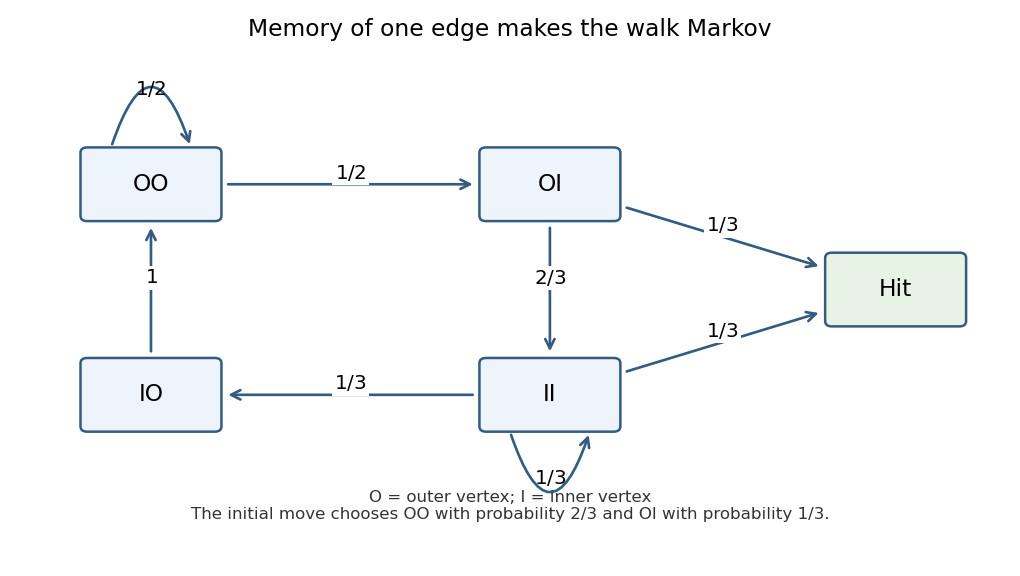
Transition probabilities between the four directed-edge types of the non-backtracking maze walk and its absorbing target
. Details. 
Let their remaining mean times be in that order. The first-step equations areSolving gives , , , . The first move from the initial outer vertex reaches type with probability and type with probability , so the intelligent starting mean isThis hitting a hub from two four-cycles calculation reduces the mean from to , saving moves. Excluding immediate reversal removes wasteful two-step returns, although it does not guarantee that the next move is toward the target.
Past exam of the mathematics course of the University of Cambridge 2009 ib Paper 1 18H Solution Created 2026-09-24 Updated 2026-10-14
A critical region is the set of sample outcomes on which a test rejects its null hypothesis. Its power function is ; its size of a statistical test is . Randomized tests replace the indicator of by a rejection probability .
The Neyman-Pearson lemma states that for two simple hypotheses with densities , the test that is one where , zero where , and randomized on equality to have null rejection probability , maximizes power among tests of size at most . Here . To prove it, let be any competing test. Pointwise, , since both factors have the same sign off the equality set. Integrating givesThis proves the lemma, including equality-set randomization and points where .
Take the exponential parameter to be its rate: for . For , the joint likelihood ratio is , decreasing in . Hence for the most powerful test isThere is no boundary randomization because has a continuous gamma distribution. Its density follows by repeated convolution: . Integrating by parts gives the exponential-rate likelihood-ratio test powerThe threshold is the unique positive solution of this formula at with value . Differentiating the finite sum yieldsThus the power function is strictly increasing, and its supremum over is . Therefore the same test has size for the composite null . Since the threshold does not depend on the particular larger rate, it is also uniformly most powerful against all . The endpoint sizes zero and one have their trivial constant tests.
Past exam of the mathematics course of the University of Cambridge 2009 ib Paper 1 17D iii Created 2026-09-24 Updated 2026-09-24
Past exam of the mathematics course of the University of Cambridge 2009 ib Paper 1 17D ii Created 2026-09-24 Updated 2026-09-24
Past exam of the mathematics course of the University of Cambridge 2009 ib Paper 1 17D i Created 2026-09-24 Updated 2026-10-14
Past exam of the mathematics course of the University of Cambridge 2009 ib Paper 1 16A c Created 2026-09-24 Updated 2026-09-24
Past exam of the mathematics course of the University of Cambridge 2009 ib Paper 1 16A b Created 2026-09-24 Updated 2026-09-24
Past exam of the mathematics course of the University of Cambridge 2009 ib Paper 1 16A a Created 2026-09-24 Updated 2026-09-24
Past exam of the mathematics course of the University of Cambridge 2009 ib Paper 1 15B Solution Created 2026-09-24 Updated 2026-10-14
The parity operator acts by . For an even potential, differentiating twice and using proves on the parity-invariant domain of the Hamiltonian operator. Therefore each energy eigenspace is invariant under . The projectors and split it into even and odd subspaces, giving a basis of simultaneous eigenstates. An odd state obeys , hence .
The infinite walls impose , with the wavefunction zero outside. It is continuous at the central delta potential. Integrate the stationary Schrödinger equation over ; the energy integral tends to zero and the Dirac delta function contributes . This givesFor the given piecewise positive-energy form, . Replacing by swaps the two pieces and leaves their values unchanged, proving . The value at zero is , and the one-sided derivatives are and . The jump condition gives . The wall at gives , henceFor the undivided wall equation instead gives the usual free even roots. For , set and . In every interval there is exactly one root: writing gives , whose two sides are respectively strictly decreasing and increasing. These are all positive even roots; the quadratic form is nonnegative, so there are no negative eigenvalues. Thus and .
The printed limit of this absolute energy difference is false. The exact quantization equation gives , so but . ConsequentlyThus the high-energy shift from a central delta barrier is a finite positive constant, not zero. The corrected vanishing statement is the relative shift , or the wave-number difference . Physically, highly energetic particles are weakly affected in relative terms by a fixed point barrier. The free even wavefunction normalized in has density at the origin, so the barrier's first-order expectation is , matching the exact limit.
Odd states vanish at zero, so the delta term and the derivative jump both vanish. Their normalized wavefunctions and energies arewith zero wavefunction outside. They do not depend on . These even and odd sectors describe the central delta barrier in a symmetric infinite well.
Past exam of the mathematics course of the University of Cambridge 2009 ib Paper 1 14B Solution Created 2026-09-24 Updated 2026-10-14
Write with . Substitution into the ordinary differential equation givesUnless the series terminates, its coefficient ratio is , so it converges for every finite . A coefficient first vanishes exactly when is a nonnegative integer , and then , . Thus is a polynomial precisely for , in which caseis the normalized Laguerre polynomial.
Multiplying the differential equation by gives . Multiply by , subtract the equation with the indices exchanged, and integrate over . The boundary term vanishes both at zero and infinity. ThereforeThis is the weighted orthogonality of the Laguerre polynomials.
Their leading coefficients show . Since have distinct degrees, they form a basis of that polynomial space. Hence , and comparison of leading coefficients gives . Likewise the degrees of and for run through and , respectively. A nontrivial linear combination cannot cancel its highest-degree term, so these functions are linearly independent.
For , this gives the basis of the cubic polynomial space, establishing the specified expansion. Its weighted integral is : integrates to one, and are orthogonal to , and integrates to zero. At the two roots of , the expansion reduces to . Solving these two equations for givesFor explicit verification, the recurrence gives , . Thus , are distinct positive roots and , . This is the two-node Gauss-Laguerre quadrature rule, exact for every cubic.
Past exam of the mathematics course of the University of Cambridge 2009 ib Paper 1 13D Solution Created 2026-09-24 Updated 2026-10-14
Choose the principal branch of a multivalued function, , for . The integrand has simple poles at and a branch cut along the negative real axis. Its residues arewhose sum is .
For , close the Bromwich contour to the left using a rectangle with outer real part and horizontal edges at imaginary parts , indenting the cut and zero. On every distant edge, , and . Each edge has length and , so its integral is . The small circle of radius about zero contributes . The tails of the original vertical integral are absolutely bounded by as well.
On the upper and lower banks at , the square roots are and , respectively. With the upper bank traversed toward zero and the lower bank away from zero, their combined integral isThe cut integral converges near zero since is integrable, and at infinity by exponential decay. The residue theorem, followed by and , therefore givesFor , close the Bromwich contour to the right. There are no enclosed poles or cuts, and there. The same distant-edge estimates show for .
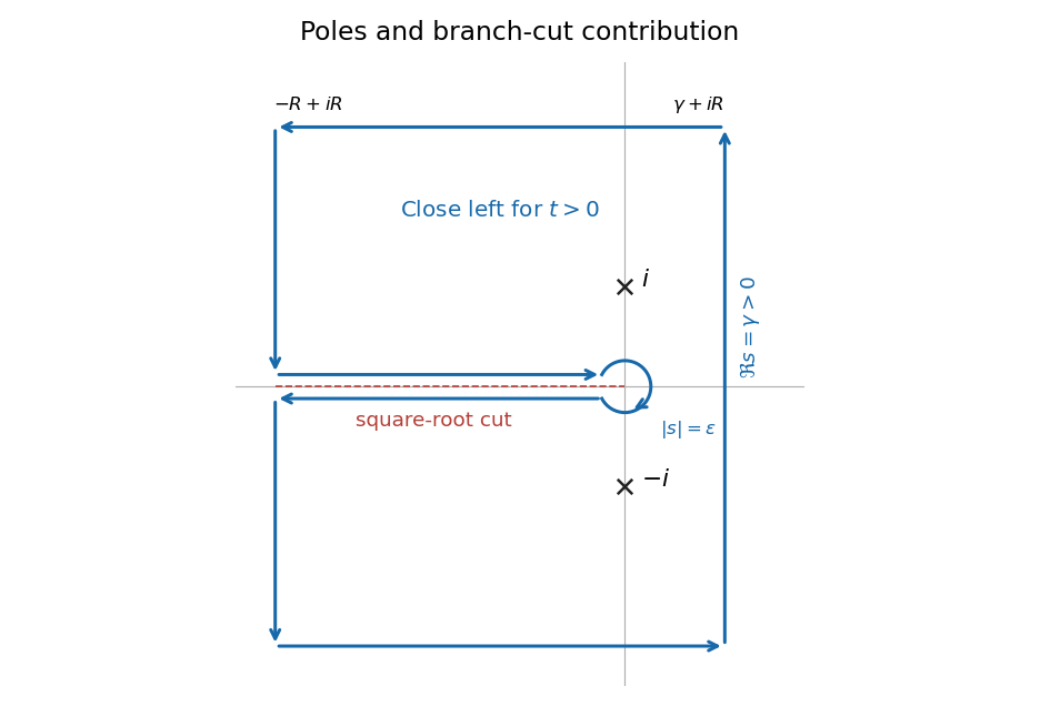
Left-closing Bromwich contour with the principal square-root cut, two pole residues, and a small indentation at zero
. Details. 
For the large- expansion, . Scaling and using the given integral yields . Integration by parts twice gives the next coefficient . The remainder is bounded by . Thus, without needing a globally convergent termwise integration of the local power series,In particular, the requested two leading terms are , interpreted as an additive asymptotic expansion. This is Bromwich inversion with a square-root branch cut.
There are unlisted articles, also show them or only show them.