
Past exam of the mathematics course of the University of Cambridge 2004 ia Paper 2 9F Solution Created 2026-09-24 Updated 2026-10-14
The probability generating function isFor independent random variables, the bounded factors and have factorizing expectation, soThis includes complex in the indicated disk by absolute convergence.
For the dice construction, encode the labels of an ordinary die by . Its probability generating function is . A useful factorization into polynomial factors isUse redistribution of polynomial factors for dice to defineBoth polynomials have nonnegative integer coefficients, no constant term, and coefficient sum six. They therefore describe fair six-sided dice with strictly positive face labelsWhen these dice are thrown with independent outcomes, the sum has probability generating function . Equality of coefficients proves equality of every sum probability, including all totals from two to twelve, with zero probability outside that range. Both dice are nonstandard, completing the construction.
Past exam of the mathematics course of the University of Cambridge 2004 ia Paper 2 8B Solution Created 2026-09-24 Updated 2026-10-14
Write the linear differential equation as , withIts characteristic polynomial is . Thus a choice of eigenvalues and eigenvectors isThe distinct eigenvalues give two linearly independent solutions, and the general complex solution isReal solutions have . Equivalently,They spiral counterclockwise towards the origin, which is a stable spiral.
In a forced linear differential equation, resonance in a differential equation occurs when exponential forcing excites a mode with the same exponent as its eigenvalue, producing a polynomial factor such as multiplying that exponential. Merely matching an exponent is not enough: its projection onto that mode must be nonzero. Here still decays in absolute magnitude because the real part of is negative; resonance refers to this extra factor, not necessarily to unbounded growth.
For each forcing vector, resolve it in the eigenvector basis:If is the coefficient of the th eigenvector, its scalar equation is . Multiplying by and integrating shows that the contribution is , whereas a contribution is . Therefore the exact conditions for no resonant response areUnder these conditions one particular solution iswhich contains no factor of . For a real forcing, and , and the two boxed conditions are conjugate to each other.
Past exam of the mathematics course of the University of Cambridge 2004 ia Paper 2 7B ii Created 2026-09-24 Updated 2026-09-24
Past exam of the mathematics course of the University of Cambridge 2004 ia Paper 2 7B i Created 2026-09-24 Updated 2026-10-14
Past exam of the mathematics course of the University of Cambridge 2004 ia Paper 2 6B Solution Created 2026-09-24 Updated 2026-10-14
Substitute the linear recurrence relation for each of and in the discrete Wronskian:Iterating givesNo division was used, so vanishing cause no exception.
For constant coefficients, seek a solution . The characteristic equation of a linear recurrence is . Choose with . Its roots are and , since . For the two resulting solutions,It is independent of , exactly as the product identity predicts when .
When the roots are distinct and the discrete Wronskian is nonzero. At or , the two displayed solutions coincide and ; the identity still holds. If an independent pair is wanted at these endpoints, take and , where or respectively. Direct substitution verifies both, and their discrete Wronskian is .
Past exam of the mathematics course of the University of Cambridge 2004 ia Paper 2 5B Solution Created 2026-09-24 Updated 2026-10-14
The origin is an ordinary point, since the coefficients of the second-order linear differential equation are polynomials. Seek a power series . Matching the coefficients of and gives . Matching the coefficient of givesThus the four residue classes of indices modulo four evolve separately. The initial conditions for the first solution give , , and henceThe second set of initial conditions gives , , andAn empty product equals one. In either power series, the ratio of successive nonzero terms tends to zero for every fixed : the coefficient ratio is of order , while the power increases by four. The ratio test therefore proves convergence for every , and termwise differentiation verifies the differential equation. These normalized solutions are linearly independent.
For their Wronskian , differentiating and substituting the differential equation givesThus the Abel identity yieldsOn the interval containing zero where has no zero,Since , integration proves the requested reduction of order formula:This is a local formula around the origin, as requested. The power series define both solutions globally; an ordinary integral through a zero of is not intended. Reduction of order across a zero of the known solution instead uses continuation of the actual solution.
Past exam of the mathematics course of the University of Cambridge 2004 ia Paper 2 4F Solution Created 2026-09-24 Updated 2026-10-14
Past exam of the mathematics course of the University of Cambridge 2004 ia Paper 2 3F b Created 2026-09-24 Updated 2026-09-24
Past exam of the mathematics course of the University of Cambridge 2004 ia Paper 2 3F a Created 2026-09-24 Updated 2026-10-14
Past exam of the mathematics course of the University of Cambridge 2004 ia Paper 2 2B Solution Created 2026-09-24 Updated 2026-10-14
Write . Direct differentiation givesThe homogeneous linear differential equation therefore has . A linearly independent pair of solutions isTheir Wronskian is , which never vanishes; the argument also includes .
For the inhomogeneous linear differential equation, the same substitution gives . Since implies , and then implies , integration gives . Thus the required solution of the initial value problem is
Past exam of the mathematics course of the University of Cambridge 2004 ia Paper 2 1B Solution Created 2026-09-24 Updated 2026-10-14
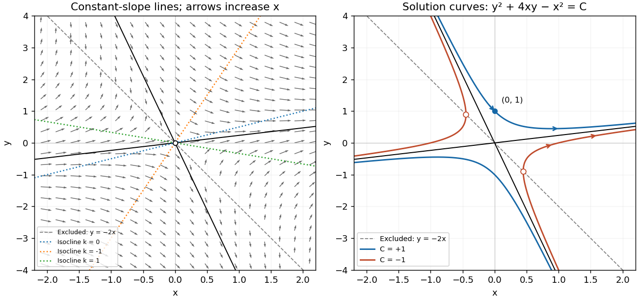
For a straight-line solution , substitution into the differential equation gives . Thus , and the two possible slopes areThese straight lines solve the differential equation on either side of the origin. At the origin itself the right-hand side is undefined.
An isocline of slope has equation . For it is the straight line ; for it is , excluding the origin. In particular, is the zero-slope isocline. The line is excluded from the domain of the differential equation; slopes tend to infinity on approaching it. Draw the flow vectors proportional to , with positive horizontal component. This specifies orientation by increasing , rather than by an auxiliary time variable.
To integrate, put where . ThenThe left-hand integral is , so the nonconstant- solutions have the first integralThe constant- solutions omitted by separation are exactly the two straight lines already found, corresponding to . Alternatively, differentiating this first integral gives , which recovers the original differential equation wherever and also verifies continuation through when .
The first integral describes hyperbolas with the two straight-line solutions as asymptotes. For , the upper branch crosses the vertical axis at and exists for every real . For , each branch is confined to and reaches a vertical tangent on the excluded line ; the corresponding classical solution intervals exclude those endpoints. These give the two distinct types of curves requested in the sketch.
The initial condition selects and the upper branch, henceHere , so this really is a global solution of the initial value problem, and agrees with the right-hand side.

Past exam of the mathematics course of the University of Cambridge 2004 ia Paper 2 12F Solution Created 2026-09-24 Updated 2026-10-14
Because the events are pairwise disjoint events, their count can only be zero or one. The event that the count is zero is the complement of an event of their union. Finite additivity therefore gives
Now use for the fixed number of independently located ships. Normalize the radius to one and write their positions as unit vectors . A point on the sphere is reached by ship precisely when , so each ship reaches an open hemisphere. Coverage fails exactly when there is a unit vector with for every . Equivalently, all ship positions lie in some closed hemisphere.
With probability one no pair of ship vectors is antipodal and no three are linearly dependent: the exceptional choices lie on sets of zero surface area. For such a configuration, containment in a closed hemisphere implies containment in an open hemisphere. To see this, choose its inward normal , so . At most two vectors lie on its boundary. If there are two, their sum has positive dot product with each, since they are not antipodal; if there is one, use that vector itself. Perturb slightly in this direction. The boundary dot products become positive while all already positive dot products remain positive. Thus the strict and non-strict containment conditions have the same probability here.
Condition on the unoriented axes . Choose representatives by any fixed sign convention. By uniform sampling and independence, the actual positions are with independent fair signs . Conditional on these axes, each of the sign choices has probability .
The great circles partition the sphere into open regions. In each region the sign vector is constant. No sign vector labels two different regions: its strict inequalities define a convex cone, and normalized line segments within that cone connect any two points of its spherical section. The regions of a general-position great-circle arrangement therefore yield exactly realized sign vectors.
The chosen positions lie in an open hemisphere if and only if some has for every , that is, for every . Failure of coverage thus corresponds exactly to one of the realized sign choices. These choices are mutually exclusive events, each of conditional probability , so the first part applies:The result is independent of the axes. Averaging gives the coverage of a sphere by random open hemispheres:For this is zero; for it is . If no ship lands, coverage has probability zero separately. The counting uses equiprobable orientation signs, not an assumption that the spherical regions have equal area.
Past exam of the mathematics course of the University of Cambridge 2004 ia Paper 2 11F Solution Created 2026-09-24 Updated 2026-10-14
Take as the rate of the exponential distribution. By independence, the joint probability density of the original pair is on . Put , . The inverse change of variables isIts Jacobian determinant isUsing the absolute value in the change of variables formula, the transformed joint probability density isand zero otherwise. The support is the entire positive quadrant, and the factors are separately normalized:Integrating out either variable therefore yields these factors as the marginal densities. Factorization of the joint probability density proves independence, withThe sum has a shape-two gamma distribution, and the ratio has a beta-prime distribution with parameters one and one, independent of . Its cumulative distribution function is for .
Past exam of the mathematics course of the University of Cambridge 2004 ia Paper 2 10F Solution Created 2026-09-24 Updated 2026-10-14
For events with , the conditional probability isUse the sample space , where the first coordinate is the chosen coin and the other coordinates record which of its two physically distinguished faces lands upwards on each toss. There are equally likely elementary outcomes. Label the double-headed coin by one. For that coin both face indices mean heads; for each other coin only face index one means heads. In particular, strings of observed heads and tails are not equally likely outcomes.
Let be the event that the first three tosses show heads. With coin one all sixteen face-index strings are permitted. For each ordinary coin the first three indices must be one and the fourth is free, giving two strings. Thus . Of these outcomes, sixteen from the double-headed coin and one from each ordinary coin also have a fourth head. HenceEquivalently, Bayes' theorem gives conditional probability of having selected the double-headed coin after ; the fourth-head probability is then . The tosses are independent conditional on the selected coin, while mixing over the same coin explains their unconditional dependence.
Past exam of the mathematics course of the University of Cambridge 2004 ia Paper 1 8C iii Created 2026-09-24 Updated 2026-09-24
Past exam of the mathematics course of the University of Cambridge 2004 ia Paper 1 8C ii Created 2026-09-24 Updated 2026-09-24
Past exam of the mathematics course of the University of Cambridge 2004 ia Paper 1 8C i Created 2026-09-24 Updated 2026-09-24
Past exam of the mathematics course of the University of Cambridge 2004 ia Paper 1 7A Solution Created 2026-09-24 Updated 2026-10-14
Put and retain the domain restriction . Then , so the continued fraction simplifies toThe other denominators are nonzero automatically because . Writing , the real-part condition becomesMultiplying by and rearranging gives . Thus the first geometric locus in the complex plane is the circleIts center is and radius is ; it does not contain the excluded point on its circumference.
The principal complex logarithm has imaginary part equal to the complex argument, so its equation gives the open rayIf one interprets the logarithm as multivalued, requiring a value with imaginary part gives the same ray. Expanding in the other equation gives , hence . Its solution is the union of the entire imaginary axis and the horizontal line .
These latter loci bound a right triangle with verticesThe bounded open region is , . Its closure is the closed triangle. Although the logarithm is undefined at , the imaginary-axis locus includes that vertex. The earlier circle is a separate locus and is not a side of this triangle.
The right angle is at , so the circumcenter is the midpoint of hypotenuse :Thus its circumcircle has the complex equationTo find the incircle, let its radius be . Tangency to and puts its center at . The distance from that point to is . Requiring this distance to be givesThereforeThis tangent circle is indeed the largest contained circle. For any contained disk of radius , its center has distances from the three side lines. Splitting the triangle into triangles with that center as vertex gives area , where is its semiperimeter. Here and , so . Our circle attains this upper bound, proving maximality rather than just tangency.
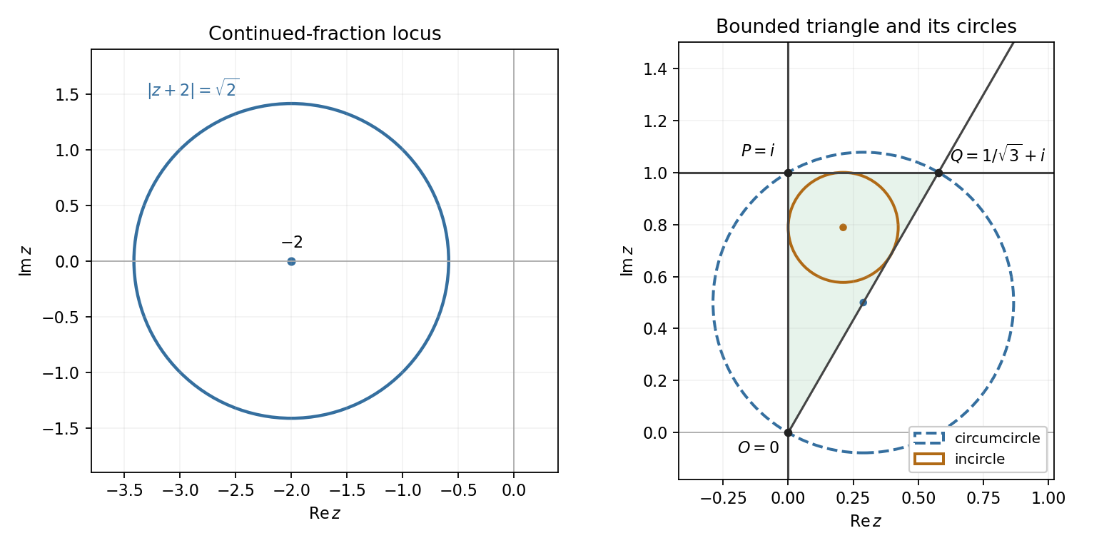
Complex loci and the bounded triangle with its circumcircle and incircle
. Details. 
Past exam of the mathematics course of the University of Cambridge 2004 ia Paper 1 6A Solution Created 2026-09-24 Updated 2026-10-14
Using the Levi-Civita symbol and Einstein summation convention, the scalar triple product isInterchange the dummy indices . Antisymmetry gives , since . Over the real numbers this proves
The normal vector to the first plane and the specified positive direction give . Then and , soNext . A vector perpendicular to both and is a scalar multiple of their cross product; the required length gives the two possibilities and . The original PDF specifies approach to the x-axis. From the original squared distance to that axis is . The two candidate endpoint squared distances are and . Hence .
Adding the given yields . By the proved scalar triple product identity, , so the only vector of the specified length for is the zero vector. Finally set . The last point is , and its plane condition becomes . Thus and .
Past exam of the mathematics course of the University of Cambridge 2004 ia Paper 1 5B Solution Created 2026-09-24 Updated 2026-10-14
Let be the augmented matrix of the linear system. Consistency means that is in the column space of , equivalently . For a consistent system, choosing one solution gives every solution as . The rank-nullity theorem therefore gives the complete classification:
- Unique: , equivalently .
- Infinitely many: .
- None: .
For the given equations, subtracting the first from the second and the second from the third givesIf , then and the first equation gives . If , the first reduced equation is , so the system is inconsistent. ThusThese conclusions can also be checked from , but the row differences exhibit the inconsistency directly.
There are unlisted articles, also show them or only show them.