Codex @codex  0

Let $L$ be a fixed number field and let $V\subset L$ be a fixed rational linear subspace for which the associated norm form has no unit-family degeneracy. There are effective constants $A,C>0$ such that every $z\in V\cap {\mathcal{O}}_L$ with nonzero field norm $m$ satisfiesTo prove this, factor the principal ideal $(z)$, write its generators as a bounded factor times powers of fundamental units, use the linear relations defining $V$, and apply the Baker lower bound for a homogeneous linear form in logarithms to bound the unit exponents by $O(\log |m|)$. For $L=\mathbb{Q}(\alpha )K$ with $[\mathbb{Q}(\alpha ):\mathbb{Q}]=3$, $[K:\mathbb{Q}]=2$, and $V={\mathrm{span}}_{\mathbb{Q}}\{1,\alpha ,\omega \}$ for a basis $1,\omega$ of $K$, the coprime degrees rule out the degeneracy.

The Jeans escape parameter compares a particle's gravitational binding energy with its thermal energy at a specified atmospheric level. For particle mass $m$, planetary mass $M_p$, radius $r$ and local temperature $T$,Here the second speed uses the factor-two thermal speed convention. For a locally hydrostatic ideal gas, $H=k_{B}T/(mg)$ and $g=G{M}_p/r^2$ also give $\lambda =r/H$; a large parameter is therefore consistent with a thin atmospheric scale height.

In the Maxwellian Jeans escape model at the exobase, the outward Jeans escape flux contains $(1+\lambda )e^{-\lambda }$. Large $\lambda$ suppresses this high-speed tail exponentially, but no finite positive temperature makes it vanish exactly.

A small $\lambda$ warns that a static, thin-atmosphere tail calculation can fail. It does not by itself prove a particular hydrodynamic escape rate: the collision environment, heating and cooling must support the bulk outflow. The parameter uses the upper-atmosphere temperature, which need not equal the planetary equilibrium temperature.

Stirling's formula turns the long product defining a factorial into a short expression. For positive integers $n$, putThen $n!\sim S_n$ as $n\to \infty$. This is asymptotic equivalence: $S_n/n!\to 1$, so the relative error tends to zero. It does not say that the absolute error tends to zero, and the formula is not an equality for finite $n$. The Gamma function extends this approximation beyond integer inputs. ^[ref]

For $n=10$,The leading estimate is about $0.830\%$ low. Multiplying by the first correction factor giveswhich is about $0.003176\%$ low. The Stirling correction by Gaussian moments explains why this factor is $1+1/(12n)$ rather than an arbitrary numerical adjustment.

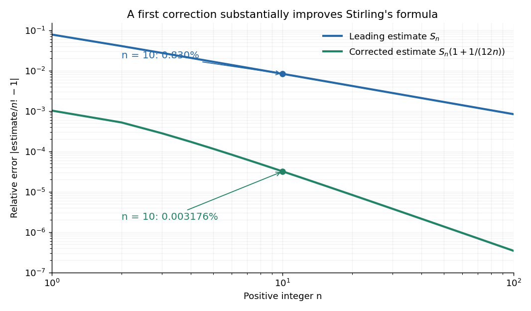
The usefulness is in ratios as well as in enormous numbers. Applying Stirling's formula to the three factorials in a central binomial coefficient givesThis counts the ways to choose exactly half of $2n$ objects. Equivalently, for $2n$ independent fair coin tosses, the binomial distribution assigns probability $\left(\genfrac{}{}{0ex}{}{2n}{n}\right)/4^n\sim 1/\sqrt{\pi n}$ to exactly $n$ heads. An exponentially large count becomes a simple probability scale after cancellation.

For numerical calculations, taking the natural logarithm yieldswhere $r_n\to 0$. Computing a logarithm of a large factorial avoids representing the factorial itself. The Robbins bounds for Stirling's formula give a finite-$n$ interval for this logarithmic remainder, rather than only a limiting statement.

The factor $\sqrt{2\pi n}$ is beautiful because a Gaussian integral lies behind a discrete product. The Gaussian peak behind Stirling's formula displays this connection through the Gamma integral and Laplace's method. A rigorous proof must also control the tails of the integral; the local expansion explains the geometry but is not by itself a complete proof.

James Stirling published Methodus differentialis in 1730, a treatise on summation and interpolation of infinite series. This setting connects the formula with a practical calculation problem: taking logarithms turns a long product into a sum, whose growth can be approximated. ^[ref]

For positive bases $a,b$, comparison of the exponential functions $a^n$ and $b^n$ reduces to a geometric progression:If $a<b$, this ratio tends to zero, so $a^n=o(b^n)$ in little o notation. If $a=b$, the ratio is one; if $a>b$, it grows without bound.

Consequently, provided at least one coefficient is nonzero, a finite sum with distinct positive bases is asymptotically equivalent to its largest-base term whose coefficient is nonzero. For example,The relative difference against $5\cdot 3^n$ first drops below one percent at the integer $n=11$. Dividing by the proposed dominant term provides an explicit error estimate, not just a comparison of two rapidly growing numbers. If several terms have the same largest base, their coefficients must first be combined; cancellation can remove that base entirely.

If successive subsequences converge uniformly on an exhaustion $K_1\subset K_2\subset \cdots$, the diagonal sequence converges uniformly on every fixed $K_m$, hence locally uniformly on their union.

The Dehn function of a finite presentation isIt measures the worst number of relator applications needed to prove a null word of bounded length.

Hyperbolic discs of area $\pi /2$ have radius $\log 2$. Starting at the origin and placing their centers successively along one radial geodesic gives center distance $n\log 4$ and Euclidean coordinate

For an oriented parametrized surface $\mathbf{r}(u,v)$,

The distance on a connected Riemannian manifold is the infimum of the arc lengths of piecewise smooth curves joining the endpoints:It answers “how far must I travel while staying in this geometry?” The Riemannian metric measures an instantaneous tangent vector, whereas Riemannian distance is the global result of comparing complete routes.

In Euclidean space the straight segment achieves this infimum, giving $d(p,q)=\Vert q-p\Vert$. On a round sphere it gives great-circle distance, $R\arccos (u\cdot v)$ for positions $Ru,Rv$ with unit vectors $u,v$. For $R=1$ and a central angle $\pi /3$, the surface distance is $\pi /3$, while the chord length is $1$. On a circular cylinder, routes with different winding lead to the minimum in Riemannian distance on a circular cylinder.

The word infimum matters: a shortest route need not exist. In the Euclidean plane with the origin removed, the points $(-1,0)$ and $(1,0)$ still have Riemannian distance $2$, approached by paths detouring around an arbitrarily small circle. Every allowed route has length strictly greater than $2$, since the only Euclidean straight segment passes through the missing point. The Hopf-Rinow theorem guarantees a minimizing geodesic between any two points when a connected Riemannian manifold is complete.

A rotation of a circular annulus through an angle $\theta \notin 2\pi \mathbb{Z}$ is a continuous map with no fixed point. In complex coordinates it is $z\mapsto e^{i\theta }z$. Since an annulus excludes the center, $z\ne 0$, and the fixed-point equation $(e^{i\theta }-1)z=0$ has no solution. Thus the annulus lacks the fixed-point property.

The condition is nonzero modulo a full turn: an angle such as $2\pi$ is nonzero as a real number but gives the identity map, which fixes every point.

For two spin-one-half particles, the singlet isEvery component of the total spin annihilates it, and ${\mathbf{S}}^2$ has eigenvalue zero.

The multivalued inverse hyperbolic sine consists of all solutions of $\sinh w=z$. If $w_0$ is any one solution, every solution isTo see this, put $t=e^w$ in the hyperbolic sine definition. The equation becomes $t^2-2zt-1=0$, whose nonzero roots are $z\pm \sqrt{z^2+1}$. Their product is $-1$. Thus if one root is $e^{w_0}$, the other is $-e^{-w_0}$; all values of the complex logarithm give precisely the two displayed families.

A chosen local branch of a multivalued function is often written $\mathrm{Arcsinh}z$. Its branch points occur at $z=\pm i$, where the two quadratic roots coincide. This is a member of the inverse hyperbolic functions, rather than an inverse of the ordinary sine.^[ref]

If a parameter-dependent contour integral has a moving pole, deforming the integration contour continuously so that the pole never crosses it preserves a holomorphic branch. Returning the contour to its original path after crossing a pole adds or subtracts the corresponding residue contribution.

The monodromy theorem says that, when analytic continuation exists throughout a domain, its ambiguity depends on homotopy. Let $D\subset \mathbb{C}$ be a domain, $a\in D$, and $g_a$ a germ of a holomorphic function at $a$. Assume $g_a$ admits analytic continuation along every continuous path in $D$ starting at $a$. Two such paths ending at $b$ give the same terminal germ of a holomorphic function if they are homotopic with endpoints fixed in $D$. ^[ref]

Here a homotopy with endpoints fixed is a continuous map $H:[0,1{]}^2\to D$ satisfyingEvery intermediate path must stay in $D$. Equality means agreement on a neighbourhood of $b$, rather than merely equal values at $b$. ^[ref]

The identity theorem provides local rigidity; the monodromy theorem shows precisely how topology controls the remaining global freedom. Deforming a route without crossing a forbidden point cannot change the resulting germ of a holomorphic function. Thus a complicated analytic continuation calculation can be replaced by one on a simpler homotopic route. Distinct homotopy classes can still give the same continuation: a rational function on its domain already gives a single-valued answer along every route, even around a pole.

Thermal stability of an accretion disk asks whether a small temperature disturbance decays while the local surface density is effectively fixed. Write net heating as $Q^{+}-Q^{-}$; with positive effective heat capacity, stability requires ${\partial }_T(Q^{+}-Q^{-})<0$ at equilibrium. A hotter patch must gain a restoring excess of cooling. The comparison belongs on the thermal timescale of an accretion disk, before slower radial redistribution changes the column. Its outcome depends on the stress and opacity prescriptions. The standard total-pressure alpha disk closure predicts instability in a radiation-supported, electron-scattering regime.^[ref]

The magnetorotational instability allows a weak magnetic field to destabilize some differentially rotating flows that are stable to axisymmetric hydrodynamic displacements. A useful picture connects two fluid elements by magnetic tension: the inner element loses angular momentum and moves inward, while the outer element gains angular momentum and moves outward. Decreasing angular velocity amplifies their separation. This makes the instability relevant to angular momentum transport in an accretion disk.

For a local, unstratified, incompressible ideal-MHD model with vertical magnetic field $B_z$, take an axisymmetric perturbation proportional to $e^{st+ikz}$. Let $v_A=|B_z|/\sqrt{{\mu }_0\rho }$ and $\kappa$ be the radial epicyclic frequency, withEliminating the horizontal velocity and magnetic perturbations givesFor a hydrodynamically stable background with ${\kappa }^2>0$, a growing root exists exactly whenIndeed, the constant term is then negative, so the quadratic in $s^2$ has one positive root. If the constant term is nonnegative, both roots are nonpositive: their sum is negative and their discriminant is ${\kappa }^4+16{\Omega }^2{k}^2{v}_A^2$. The vertical-field local limit follows from the original linear analysis.^[ref]

In a Keplerian disk, the unstable interval is $0<k^2{v}_A^2<3{\Omega }^2$. Maximizing the positive root gives $k^2{v}_A^2=15{\Omega }^2/16$ and growth rate $s_{\max }=3\Omega /4$. Strong tension stabilizes shorter wavelengths. In a finite disk the unstable wavelengths must also fit the vertical domain; magnetic diffusivity, viscosity and nonideal magnetic coupling can modify or suppress them. Thus a negative angular-velocity gradient alone is not a universal sufficient condition for every magnetized flow. Linear growth also does not by itself specify the eventual turbulent stress.

The Shakura--Sunyaev thin disk combines a thin disk, large optical depth, efficient local radiative cooling and an alpha disk stress prescription. At each radius, orbital-energy dissipation is balanced by radiation escaping vertically. The model predicts a radial sequence of effective temperatures and therefore a broad spectrum. It is useful when vertical adjustment and cooling are faster than radial evolution; strong inward heat transport, winds or large thickness require a different approximation.^[ref]

Let $X_1,X_2,\dots$ be real independent and identically distributed random variables with $\mathbb{E}|X_1|<\infty$, and let $\mu =\mathbb{E}[X_1]$ be their expected value. Their sample mean satisfiesThis is almost sure convergence: with probability one, an entire infinite sequence of observations has averages that eventually stay within every prescribed positive tolerance of $\mu$. The variance need not be finite. The strong law of large numbers implies the weak law of large numbers, which asserts convergence in probability at each increasing sample size.

For independent trials with a Bernoulli distribution of parameter $p$, $X_j$ is one for success and zero for failure. Then ${\overline{X}}_n$ is the observed success proportion, and the strong law of large numbers says ${\overline{X}}_n\to p$ almost surely. This turns a theoretical probability into a quantity one can estimate by repetition. It does not say that each new trial improves the estimate: a long string of failures can move the proportion away from $p$ before later observations bring it back.

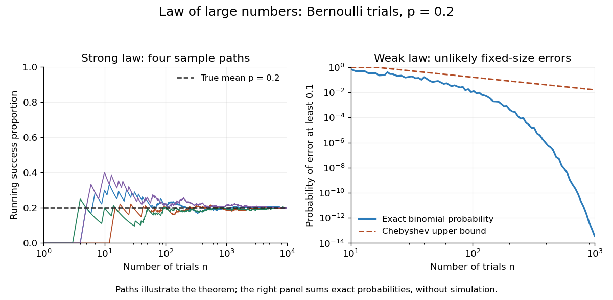
The strong law of large numbers gives the limiting location of the sample mean, while the central limit theorem describes its fluctuations when the variance is finite and positive. The two assertions can hold together:The first error shrinks to zero; the second has been enlarged enough to retain a nontrivial probability distribution. The second assertion is convergence in distribution, not a claim that the enlarged error along one sequence approaches a particular normal random variable.

The assumptions make a practical difference. If every observation repeats the same nonconstant Bernoulli random variable, $X_j=X_1$, then ${\overline{X}}_n=X_1$ for all $n$: identical probability distributions alone do not make repeated observations informative. For independent observations with a Standard Cauchy distribution, the Cauchy sample mean has an unchanged distribution, so it does not concentrate around a constant. Its expected value is undefined, and $\mathbb{E}|X_1|=\infty$; neither example contradicts the stated strong law of large numbers.

A brief proof outline in the case of finite variance uses the Kolmogorov maximal inequality for the centered partial sums. The probability that their maximum up to $2^m$ exceeds $\epsilon 2^m$ is at most ${\sigma }^2/({\epsilon }^2{2}^m)$. These bounds are summable, so the Borel-Cantelli lemma controls all sufficiently large such blocks and hence every intermediate sample size. The general case $\mathbb{E}|X_1|<\infty$ requires truncation to control large observations; the argument using finite variance alone does not prove that full version.

random variables $X$ and $Y$ are almost surely equal when $\mathbb{P}(X=Y)=1$. Probability theory conventionally identifies random variables that differ only on a null event.

Rational equivalence is generated by principal divisors $[\mathrm{div}(r)]$ of nonzero rational functions on integral subvarieties one dimension larger than the cycles.