
Use separation of variables, , and divide by where nonzero. A real separation constant givesso and . Normalizing the second factor to one at zero givesThe spatial ordinary differential equation has three types of real solution:Products are the separated eigenfunctions. The negative, zero and positive separation constants give trigonometric, linear and hyperbolic function forms respectively. There is no discrete quantization until boundary conditions on are supplied. Since is bounded, the envelope of decays for , grows for , and is bounded and periodic for . The scalar prefactor can also be derived by removing a variable scalar reaction rate by an integrating factor.
Take and set . The Rayleigh quotient of the trial for the quantum harmonic oscillator isIts denominator is . The kinetic numerator is times that denominator. For the remaining integral, put and useobtained from and integration by parts. Thus the compact cosine trial bound for the quantum harmonic oscillator isDifferentiation gives , so the minimizing parameter satisfiesThe quotient tends to infinity at either end of , and the two positive terms are equal at this stationary point, proving it is the global minimum. ThereforeFor comparison, the exact ground state has value . The trial is admissible for the energy quadratic form: it is continuous, has compact support, and its weak derivative is square-integrable. Its first derivative jumps at the support endpoints, so it need not belong to the smaller twice-differentiable operator domain; this does not invalidate the Rayleigh-Ritz variational principle bound.
Use the normalized eigenfunctions with the stated weighted inner product. Orthogonality gives . The corrected Sturm-Liouville problem and the vanishing boundary term giveFor a complex trial the numerator means , agreeing with the given formula for real trials. ThereforeIt is a convex combination of the eigenvalues, with equality only for a trial proportional to the lowest eigenfunction. The Rayleigh-Ritz variational principle consequently estimates by choosing a nonzero admissible trial family and minimizing this quotient over its parameters:The result is an upper bound. A more flexible trial space can lower it, while equality requires that the exact lowest eigenfunction belong to the trial space. One need not know the expansion coefficients to calculate the quotient directly from the trial function.
The original PDF has a typographical omission: its displayed equation has rather than on the right. Taken literally, it is an inhomogeneous boundary value problem, not the stated Sturm-Liouville problem. The quotient and the later eigenfunction expansion identify the intended equation, which the following derivation produces explicitly.
Choose homogeneous Dirichlet boundary conditions and a nonzero real admissible . Then because . For an endpoint-zero variation , integration by parts givesThe first variation of the Rayleigh quotient is thusBy the fundamental lemma of the calculus of variations, stationarity is equivalent toConversely, multiply this corrected eigenvalue equation by and integrate. The same boundary cancellation gives , so the first variation vanishes. This proves the requested equivalence for the intended equation. Homogeneous Neumann boundary conditions, or a Dirichlet condition at one end and a Neumann condition at the other, also eliminate the boundary term. General Robin boundary conditions would require the corresponding boundary contribution in the numerator.
Let and . The region is the first-octant portion of the ellipsoid . In cylindrical coordinates, write and . Away from the axis, the divergence isThe field is singular on the axis, so applying the classical divergence theorem there without qualification would be invalid. Instead remove and apply it to the remaining region. On the added cylindrical boundary the unit normal is , andIts area element is , so its flux is . The axial component of the field has zero dot product with this normal. The volume integral of the divergence is locally integrable, because its factor cancels the cylindrical measure. Thus removing a singular axis in a flux integral gives the desired improper surface integral with no extra axial term.
The divergence theorem now reduces the calculation toThe integral over is the area of a quarter unit disk. All boundary fluxes are interpreted as convergent improper integrals at the axis.
The azimuthal vector is automatically orthogonal to the other two. Their remaining dot product isThus orthogonal coordinates require , which integrates to . The initial value gives , and the smooth branch with isThe corresponding coordinate-vector norms are and , as in the hyperbolic parametrization of prolate spheroidal coordinates. Coordinate degeneracies on the axis and focal segment are understood.
Eliminating the angular coordinates on the requested surface givesIt is a prolate spheroid with long axis , equatorial radius , polar semiaxis , and foci .
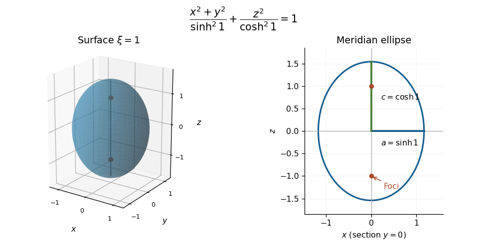

The three coordinate basis vectors are the partial derivatives of the position vector with respect to the three coordinates. Direct differentiation givesThe multivariable chain rule then gives . These are coordinate tangent vectors, not necessarily unit vectors.
A cyclic group is generated by one element: . The hypothesis needs the qualification no proper nontrivial subgroup: every nontrivial group has the proper trivial subgroup , so the literal wording admits no examples.
Under that intended hypothesis, choose . The subgroup is nontrivial and must therefore be all of , proving cyclicity. If had infinite order, then would be nontrivial and proper, since is not an even power of an infinite-order generator. Thus has finite order and .
If were composite, choose a divisor with . Then would have order , strictly between one and , again contradicting the hypothesis. ConsequentlyConversely, Lagrange's theorem shows that a group of prime order has only itself and its trivial subgroup. This proves the characterization of groups with no proper nontrivial subgroups, even without assuming finiteness at the outset.
Write . By Lagrange's theorem, the order of a group element divides four. Since no element has order four, all three nonidentity elements have order two. Thus every element is its own inverse. For any ,so the group is Abelian. Also cannot equal or , by cancellation and the fact that are distinct nonidentity elements. Hence . The remaining products are forced, givingThe map , , , preserves this table under componentwise addition modulo two. Thereforethe Klein four-group, also called the Vierergruppe.
For each , the mapis surjective by definition of a coset and injective by left cancellation. Its inverse is multiplication by . ThereforeThe same argument with right multiplication proves the analogous result for right cosets. This equality of sizes is the counting step in Lagrange's theorem.
Map each symmetry to the permutation it induces on the three vertices. This is a group homomorphism, because composing geometric motions composes their vertex permutations. In the labels chosen in (b), the map isAll six images are distinct and exhaust the symmetric group . Equivalently, the kernel is trivial because a triangle symmetry fixing all three vertices is the identity. Thus the map is bijective and
Each reflection has order two, giving exactly the three order-two subgroupsConjugation by sends to , cycling the three reflections. None of these subgroups is therefore normal.
The two nonidentity rotations generate the same order-three subgroup:It is invariant under conjugation by , and shows invariance under as well; since generate the group, this proves normality. The complete partition into conjugacy classes isThe rotations are mutually conjugate by , and the reflections by ; no rotation is conjugate to a reflection because conjugation preserves the order of a group element.
Label the triangle's vertices counterclockwise as . Let rotate it by and let reflect it in the axis through vertex 1 and the midpoint of the opposite side. ThenThe six dihedral group elements areThe first three are the identity and the rotations by ; the last three are reflections fixing vertices , respectively. These are all possible symmetries: the image of one vertex has three choices, and the order of the other two has two choices.
Use rightmost-first composition. From the generator relation,with exponents reduced modulo three and two. The row-times-column multiplication table isThus every symmetry is expressed in the two group generators .
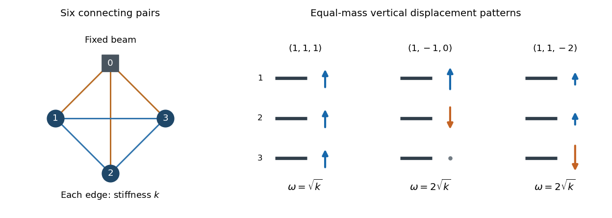
The pinned third bar has zero displacement, so remove its row and column from the stiffness matrix while retaining the springs that connect the moving bars to it. The remaining unit-mass system hasIts eigenvectors and have eigenvalues and . HenceFor these are and . The fixed value changes the static offsets and reaction force but not this linearized matrix.
For three unit masses, andThe uniform vector has , whereas every vector with coordinate sum zero is annihilated by . One orthonormal choice of normal modes is thereforeIf is retained from (b), the angular frequencies are . The equal upper frequencies follow from degenerate normal modes from permutation symmetry: the stiffness is scalar on the two-dimensional sum-zero subspace. In the uniform mode the inter-bar strings do not change length, but all three beam connections stretch, giving the nonzero lower frequency. The motion is an arbitrary sine-cosine superposition of these modes about the gravitational equilibrium.
Past exam of the mathematics course of the year 2 of the natural sciences course of the University of Cambridge 2022 Paper 2 7 a Solution Created 2026-10-18 Updated 2026-11-05
The diagram has a connection between every pair of indices , including the fixed beam . Two parallel strings, each with spring constant , together have energy . Thus the printed is the energy of a connecting pair; calling it the energy of one string would introduce a factor-of-two discrepancy.
Take vertical coordinates positive upwards, with fixed. Each bar has gravitational potential energy and kinetic energy . The Lagrangian isDifferentiating gives the Euler-Lagrange equationsEquivalently, with , the spring term is . Gravity changes the equilibrium but not the stiffness matrix. Subtracting a static equilibrium and writing gives the normal mode systemThis is the spring system underlying normal modes of an anchored complete spring graph.

There are unlisted articles, also show them or only show them.