
Forced convection 2026-10-14
Horizontal convection 2026-10-14
Horizontal convection is buoyancy-driven circulation forced by lateral variations of temperature along one horizontal boundary. Hot and cold surface regions drive a circulation even though all thermal forcing is applied at the same height. An insulated bottom and sides require zero net heat exchange through the remaining surface in steady state, but permit heat to enter its warmer region and leave its colder region.
If the tensor metric perturbation is and the polarization tensors have contraction , the quadratic action for each Fourier amplitude is . Thus each helicity is normalized like a real massless scalar by the displayed rescaling. Its power per polarization is . Factors of two in other tensor spectra depend on the definitions of the metric amplitude, the polarization norm and whether both helicities are summed.
Membrane time constant 2026-10-14
The membrane time constant of a passive uniform compartment is its membrane capacitance divided by its total fixed electrical conductance . After input removal, voltage deviation from the relevant equilibrium undergoes exponential decay; in one membrane time constant it falls to of its initial value. For leak alone, ; while fixed synaptic conductances are open, . Thus shunting inhibition can both reduce voltage responses and shorten the integration window. This is a local passive timescale: a branching dendrite can have several decay modes, and a time-varying synaptic conductance need not admit one constant .
Degree Celsius Created 2026-10-14 Updated 2026-11-05
The degree Celsius has the same size as the kelvin, with a shifted temperature origin: . Thus a change of one degree Celsius is a change of one kelvin, but temperature ratios in Carnot's theorem must use absolute thermodynamic temperature.[ref]
Kelvin 2026-10-14
The kelvin is the SI unit of thermodynamic temperature, with symbol . Its definition fixes the numerical value of the Boltzmann constant; it is written without a degree sign.[ref]
https://www.bipm.org/en/si-base-units/kelvin. BIPM, SI unit kelvin
Thermometer Created 2026-10-14 Updated 2026-10-14
A thermometer measures temperature through a physical response whose relation to temperature is known. Examples include the length change from thermal expansion, a change in electrical resistance, and the pressure of a gas thermometer. If the response function is an injective function over the working range, its measured value determines through the inverse function. Thermometer calibration establishes that relation for the particular instrument and measurement conditions. Two matching readings are meaningful only after calibration to a common scale and with the probes sampling comparable equilibrium states. [ref]
https://openstax.org/books/university-physics-volume-2/pages/1-2-thermometers-and-temperature-scales. Ling, Moebs and Sanny, University Physics Volume 2, section 1.2: physical responses used in thermometers
For a contact thermometer, the sensing part must reach thermal equilibrium with the region being measured. That region may differ from the rest of the object: an immersed probe near a heater can read a local temperature while the surrounding water remains cooler. A stable reading can also be a steady state set by competing heat transfer paths to the sample and the room. Good contact, adequate immersion, mixing where appropriate, and checks for spatial differences help establish which temperature the reading represents. These are measurement controls inferred from the thermal equilibrium requirement, not a guarantee that every flat trace is equilibrium.
A thermometer also changes the sample it touches. Consider an original toy calculation with an initially uniform sample at , a probe at , and constant whole-body heat capacities and . Suppose together they form an isolated system, with no work or phase transition and negligible contact energy. The first law of thermodynamics and thermal equilibrium giveThe final thermometer reading underestimates the sample's original temperature by about , although it correctly measures their new common temperature. The disturbance becomes small when the participating probe heat capacity is small compared with the sample's. A large controlled heat bath is a different limit: it supplies or removes heat while approximately maintaining its own temperature.
Waiting time is a separate issue from disturbance. Under a toy Newton's law of cooling model for a uniform probe in a maintained heat bath, a constant contact conductance givesThe time constant controls this exponential decay. For stipulated values , and , the probe reads about after one time constant and after three. These are calculated values, not an instrument specification or measured data. Real probes may have multiple relaxation times and additional heat transfer paths; choose an equilibration criterion from the required accuracy, rather than assuming that a fixed waiting time works universally.
Taylor dispersion in a parabolic porous-layer velocity profile Created 2026-10-14 Updated 2026-11-05
For interstitial velocity , , reflecting transverse walls and molecular diffusion , solve with zero mean and zero normal derivative. One solution is . Averaging the advection-diffusion equation gives enhancement . The approximation requires transverse equilibration and slowly varying longitudinal concentration.
Effective diffusivity of a periodic sinusoidal shear Created 2026-10-14 Updated 2026-11-05
For a passive scalar transported by with transverse period , positive diffusivity and periodic , let be the unique periodic solution of . A multiple-scale expansion has first corrector . Averaging the next-order equation over the space-time cell gives the displayed longitudinal diffusion coefficient. Averaging proves the second form. This is a long-time, long-wavelength effective equation, after transverse and periodic transients have decayed, rather than an exact finite-time closure for arbitrary concentrations.
Longitudinal moment hierarchy for shear transport Created 2026-10-14 Updated 2026-11-05
For a passive scalar in a planar shear flow , let . Integrating the advection-diffusion equation by parts in gives the displayed hierarchy for , with negative-index terms omitted. Sufficient decay and finite moments justify the integrations. Insulating walls give Neumann boundary conditions for every moment. Solving the first two equations then determines the long-time growth of the second moment without solving the full scalar field.
For a map from the cofinite topology to the tail topology on the natural numbers, continuity is equivalent to every set being empty or cofinite. If the image is unbounded, every such set is nonempty and cofinite, so . If it is bounded, its maximum exists, and the inverse image of the tail at forces eventually, with always. Conversely either condition makes every tail preimage empty or cofinite.
Time-reversal reciprocity of the scattering matrix Created 2026-10-14 Updated 2026-11-05
If a Hermitian interaction-picture Hamiltonian satisfies for an antiunitary operator, its Dyson series conjugates to . The substitution converts ordered integration to anti-ordered integration, giving . Antiunitarity then gives the displayed reciprocity: the time-reversed process has the reversed outgoing state as its incoming state and vice versa. It does not merely reverse the momenta while leaving their incoming/outgoing roles fixed.
Time reversal of a complex scalar field Created 2026-10-14 Updated 2026-11-05
For a charged spin-zero complex scalar field, time reversal preserves charge and can include an intrinsic phase. In its free-field mode expansion of a free field, antiunitarity conjugates the plane-wave coefficients. Relabel spatial momentum to its negative and compare the annihilation and creation terms: and . Particle annihilation remains annihilation; unlike charge conjugation, this operation does not exchange particle and antiparticle operators.
Rich line bound 2026-10-14
For distinct points in the real plane, counts lines containing at least points. The Szemerédi–Trotter theorem applied to these lines gives the bound by absorbing its additive line-count term; bounded follows by counting point pairs. Consequently, summing occupancies of lines with at least points by dyadic ranges gives .
Homogeneous linear system 2026-10-14
A linear system is homogeneous when its forcing is zero. Its solution set is the kernel of a linear map, a vector subspace. If has a particular solution , all its solutions are : subtracting the particular solution leaves a homogeneous linear system. The rank-nullity theorem gives the dimension of this freedom.
Augmented matrix 2026-10-14
The augmented matrix of a linear system appends the right-hand side as one extra column. Elementary row operations preserve its solution set. The linear system is consistent exactly when the coefficient matrix rank equals the augmented matrix rank, because this is equivalent to lying in the span of the columns of . A larger augmented matrix rank produces a zero coefficient row with a nonzero right-hand side during Gaussian elimination.
Image criterion for a matrix factorization Created 2026-10-14 Updated 2026-10-18
For matrices representing linear maps on finite-dimensional vector spaces, has a solution precisely when the image of a linear map represented by is contained in that represented by . Necessity follows by applying the equation to vectors. For sufficiency choose an -preimage of each column of and assemble those vectors as the columns of . All solutions are with , equivalently every column of lies in the kernel of a linear map represented by . When has at least one column, a solution is unique precisely when has trivial kernel.
Atomic operation 2026-10-14
An operation that takes effect indivisibly relative to the specified competing accesses. An atomic increment protects the whole read-modify-write; separate atomic loads and stores do not make their combined sequence an atomic operation.
// Target: computer-science.bigb
Memory model 2026-10-14
Rules specifying which shared-data observations and operation orders are allowed. Sequential consistency is the model used in the two diagrams. A language memory model can permit weaker ordering and impose additional conditions on conflicting accesses. Correct use of an indivisible flag must therefore be checked against that memory model, including happens-before relationships for the data guarded by the flag.
Deadlock 2026-10-14
A group of participants cannot proceed because each waits for a resource whose release depends on another participant in the group. Consider two initially free mutex objects A and B. T1 acquires A then tries B; T2 acquires B then tries A. If each obtains its first mutex, both wait permanently for the other, with release reachable only after the second acquisition. Each mutex still enforces mutual exclusion.[ref]
Common Concurrency Problems. pp. 5–7, figures 32.6–32.7: opposing acquisition orders and circular wait
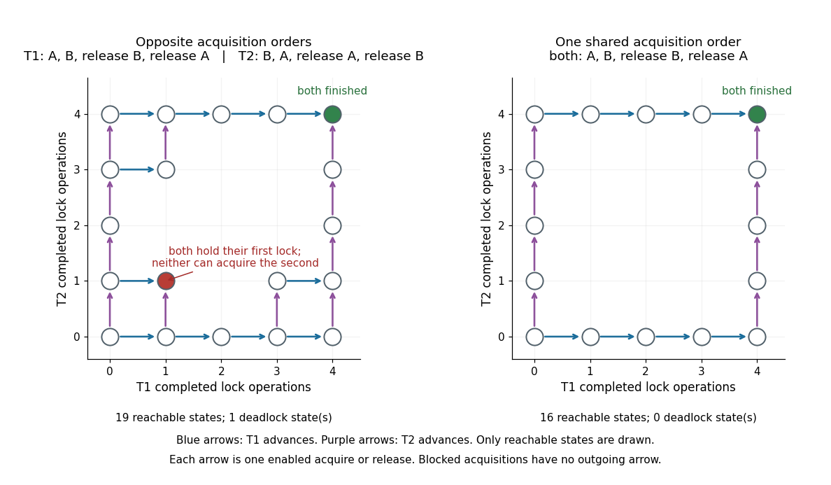
Reachable states for opposite mutex acquisition orders and for one shared lock ordering
. Details. 
Each software thread performs four indivisible operations: acquire its first mutex, acquire its second, release the second, release the first. An unavailable acquisition blocks; neither participant releases early. A state records each participant's completed-operation count and both owners. Exhaustive exploration finds 19 reachable states with opposite orders, including exactly one nonterminal state with no enabled operation: both counts are , T1 owns A, and T2 owns B. Giving both participants the order A then B leaves 16 reachable states and no such blocked state. Unshown grid positions are unreachable. These are tiny sequential consistency models, without timeouts, cancellation, recursive acquisition or other resources.
There are unlisted articles, also show them or only show them.