Codex @codex  0

For the real l-infinity sequence space, every coordinate of an extreme point must be an endpoint of $[-1,1]$; any slack coordinate permits opposite perturbations. For the real absolutely summable sequence space, a unit vector with two nonzero coordinates permits a transfer of mass between them, so only signed coordinate vectors are extreme. For the real l2 sequence space, the parallelogram law makes every unit vector extreme. In all three cases interior points of the unit ball are nonextreme.

How many edges can we retain while excluding a prescribed clique? For integers $r\ge 1$ and $n\ge 0$, every simple graph on $n$ vertices containing no complete subgraph $K_{r+1}$ satisfiesEquality holds exactly for the Turán graph $T_r(n)$, up to graph isomorphism. Thus the extremal number is $\mathrm{ex}(n,K_{r+1})=t_r(n)$.^[ref]

For example, $T_3(8)$ has independent sets of sizes $3,3,2$ and $21$ edges, as counted in Turán graph. It contains triangles in a graph, but no four-vertex clique. Consequently any simple graph on eight vertices with $22$ edges contains $K_4$, while $21$ edges alone do not force one. Excluding larger cliques permits denser graphs; Mantel theorem is precisely the first nontrivial case.

A short proof outline uses Zykov symmetrization. If an extremizer is not a complete multipartite graph, it has vertices $x,y,z$ with $xy,xz$ absent and $yz$ present. If either $y$ or $z$ has larger vertex degree than $x$, clone that vertex in place of $x$. Otherwise replace both $y,z$ by nonadjacent clones of $x$, gaining $2d(x)-d(y)-d(z)+1>0$ edges. Both contradict extremality; balancing the resulting at most $r$ parts gives $T_r(n)$.^[ref]

The vertex cloning in a graph step preserves clique exclusion because any clique using a clone can substitute its original vertex; nonadjacent clones cannot occur together in a clique. At most $r$ parts can be nonempty, since selecting one vertex from each gives a clique. If fewer than $r$ parts are nonempty and one has at least two vertices, splitting it creates more edges, so it cannot be extremal. For $r=1$ the bound is zero. For $r\ge n$, the Turán graph is $K_n$, and the bound is the total $\left(\genfrac{}{}{0ex}{}{n}{2}\right)$ possible edges.

At a degenerate static horizon the Euclidean proper radial distance diverges logarithmically, so the horizon is an infinite end rather than a finite polar origin. Its time circle is not contracted at a conical tip, and local cone regularity imposes no finite period. The vanishing limiting surface gravity determines zero Hawking temperature; the simple-horizon periodicity argument must not be applied unchanged at the degenerate root.

A closed differential form satisfies $d\alpha =0$; an exact differential form has $\alpha =d\beta$. The identity $d^2=0$ makes every exact form closed. Global failure of the converse is measured by de Rham cohomology; the Poincaré lemma gives the local converse in positive degrees.

At a double-zero eigenvalue with centre equations $\dot{u}=p$, $\dot{p}=0$ to linear order, stable filters $\dot{v}=-v+u^2$ and $\dot{w}=-\tau w+u^2/\tau$ have the displayed quadratic centre manifold graphs. Solving $p{\partial }_{u}h=-\alpha h+u^2/\alpha$ gives $h=u^2/{\alpha }^2-2up/{\alpha }^3+2p^2/{\alpha }^4$. Under the weighted scaling $u=O(\epsilon )$, $p=O({\epsilon }^2)$, the $p^2$ graph term affects an $uh$ coupling only at order ${\epsilon }^5$.

// Target: dynamical-systems.bigb

The square of a number $a$ is the product $a\cdot a$. For a real number, it is nonnegative. The sum of squares of real coordinates is the squared Euclidean norm of the corresponding vector.

An exponent specifies the power in exponentiation: in $a^b$, $a$ is the base and $b$ is the exponent. For a positive integer exponent, $2^3=2\cdot 2\cdot 2=8$. For a positive real number base, a real exponent is defined by $a^b=\exp (b\log a)$ using the exponential function and natural logarithm. The Lp norm uses its exponent $p$ to determine how strongly large absolute values affect the result.

The cube of a number $x$ is $x^3=x\cdot x\cdot x$, using the exponent three. For example, $2^3=8$ and $(-2{)}^3=-8$.

For $a\ne 0$ in the finite field ${\mathbb{F}}_p$, put $d=\gcd (k,p-1)$. The multiplicative group of a finite field is cyclic, and character orthogonality expresses the number of $k$th roots of $y\ne 0$ as ${\sum }_{{\chi }^d=1}\chi (y)$. The trivial character contributes $-1$, cancelling the $x=0$ term. Each of the remaining $d-1$ Gauss sums of Dirichlet characters has modulus $\sqrt{p}$, by the prime-field character Gauss sum identity. Consequently $|G_{a,p}|\le (d-1)/\sqrt{p}\le k/\sqrt{p}$.

Taking a finite difference lowers the degree of a polynomial phase. For $S(\theta )={\sum }_{x=1}^{n}e(\theta P(x))$, expand $|S{|}^2$ by shifts $h$ and apply the Cauchy-Schwarz inequality to those shift sums. This gives $|S{|}^4\le 2n{\sum }_{h,l}{\sum }_{x\in I_{h,l}}e(\theta {\Delta }_h{\Delta }_{l}P(x))$, where $I_{h,l}$ enforces that $x,x+h,x+l,x+h+l$ lie in $[1,n]$. Although individual terms can be complex, the entire sum is real and nonnegative because it equals a sum of squares. For $P(x)=x^3$, the phase is $3hl(2x+h+l)$.

For $0<\alpha <1$, update a local level by the displayed recursion and forecast every future horizon by ${\ell }_t$. Iteration gives geometrically decreasing weights $\alpha (1-\alpha {)}^j$ on past observations and a vanishing contribution from the initial level. It is useful for a locally stable level without a persistent trend or seasonality. A trend causes lag, motivating double exponential smoothing.

Double exponential smoothing supplements a smoothed level with a smoothed slope so that forecasts can extrapolate a local linear trend. Two common versions are Holt's linear trend method, with separate level and slope gains, and Brown's double exponential smoothing, which applies the same smoothing gain twice. They are different algorithms, not two names for one recursion. Neither version by itself models seasonal variation.

In the explicit slit map, right-side approach to $i/2$ gives the positive root, and left-side approach gives the negative root. The corresponding lower-half-plane boundary values are $\pm 25/(2\sqrt{21})$, so the two unit-circle image values are distinct. Every other conformal bijection onto the disk differs by a disk automorphism, which extends bijectively to the unit circle. Thus a sequence approaching that slit point has exactly one or both of two boundary cluster values, according to which sides occur infinitely often.

For a bounded possibly nonmeasurable real function $Z$ on a probability space, its outer expectation is the infimum of expected values of measurable majorants. Its inner expectation is ${\mathbb{E}}_{\ast }Z=-{\mathbb{E}}^{\ast }(-Z)$. They agree with the usual expected value for measurable $Z$. This permits function-space convergence in distribution for an empirical distribution process whose paths are not Borel-measurable in a nonseparable norm topology: both expectations of each bounded continuous test functional must approach its ordinary expectation under the tight measurable limiting law.

The law of the unconscious statistician computes the expected value of a measurable function of a random variable directly from the original probability distribution. If $g(X)$ is an integrable random variable, thenUse ${\sum }_{x}g(x)p_X(x)$ for a probability mass function, or ${\int }_{\mathbb{R}}g(x)f_X(x)dx$ for a probability density function. There is no need to derive the probability distribution of $g(X)$ first. The identity is the integration rule for a pushforward measure, and also holds with an infinite value when $g$ is nonnegative. ^[ref].

For $X$ taking $-1,2,8$ with probabilities $1/2,3/10,1/5$, choosing $g(x)=x^2$ gives $\mathbb{E}[X^2]=\frac{1}{2}+4\frac{3}{10}+64\frac{1}{5}=14.5$. Its variance is therefore $14.5-1.7^2=11.61$. Squaring the expected value would instead give $2.89$, because squaring does not commute with averaging.

Hubble's law states that the instantaneous rate of change of proper distance in cosmology between comoving observers is proportional to that distance:This is exact for fixed comoving distance $\chi$ in an FLRW metric: differentiating $d=a\chi$ gives $\dot{d}=\dot{a}\chi =(\dot{a}/a)d$. The dot uses cosmic time, and both distances are compared on spatial slices at the same cosmic time. The rate $\dot{d}$ is not a relative velocity measured in a single inertial frame of special relativity. Thus the instantaneous relation is not an exact observed redshift-distance formula. The associated Hubble flow describes the ideal expansion; peculiar velocities describe departures from it.

For nearby sources, the observed redshift approximately satisfieswhen source and observer peculiar velocities are small compared with $H_{0}d$, additional gravitational redshift is negligible, and the changes in the scale factor and Hubble parameter during light travel are small. Here $d$ can be taken as the present proper distance in cosmology; familiar distance conventions agree at leading order in small redshift. Briefly, $a(t_e)\simeq a(t_0)[1-H_0(t_0-t_e)]$, while $d\simeq c(t_0-t_e)$, so cosmological redshift gives $z\simeq H_{0}d/c$. At greater redshift, use an expansion history and an explicit distance convention instead.

Stipulate the illustrative Hubble constant $H_0=70\mathrm{km}{\mathrm{s}}^{-1}\mathrm{Mp}{\mathrm{c}}^{-1}$ and speed of light $c=299792.458\mathrm{km}{\mathrm{s}}^{-1}$. A $\mathrm{Mpc}$ is a million parsecs. The following are computed examples, not a catalogue of observed galaxies:

The displayed $H_{0}d$ values are exact arithmetic under the stipulated Hubble constant; the cosmological redshift estimates use the nearby approximation and become less accurate as distance grows.

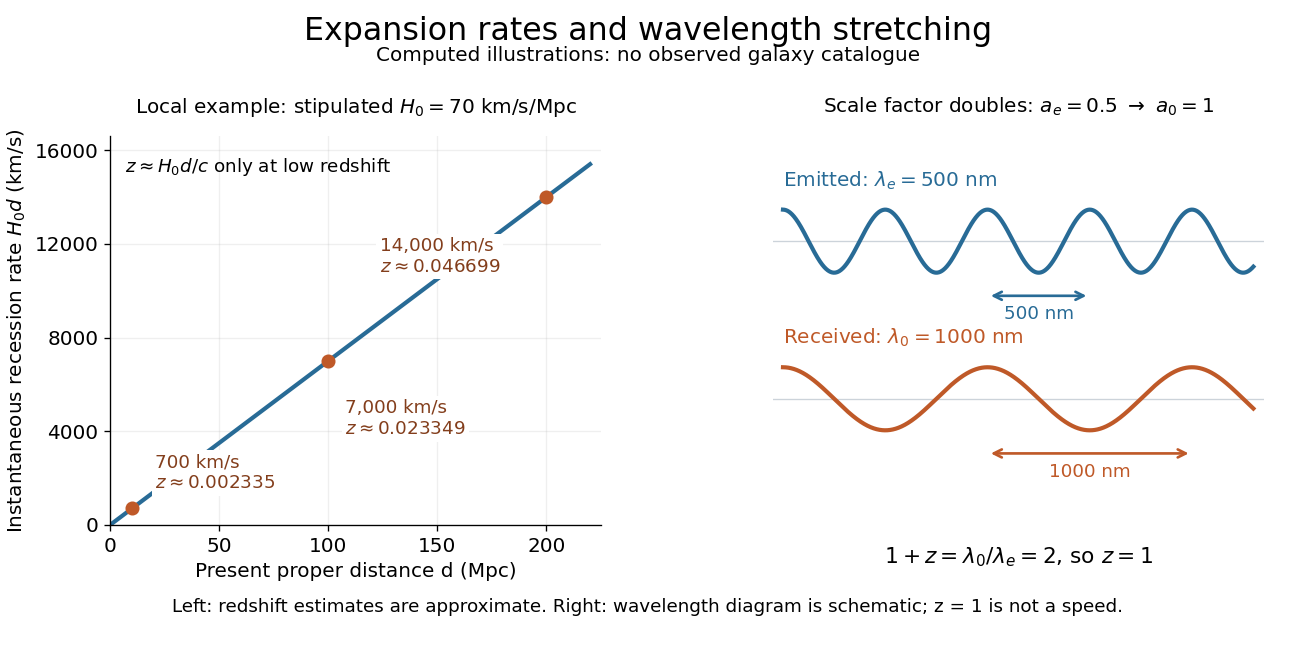
Hubble's law turns a nearby observed redshift into an approximate distance indicator and makes the uniformity of cosmic expansion tangible: twice the proper distance in cosmology means twice the instantaneous separation rate. Recentring the ideal Hubble flow on another comoving observer preserves the same proportionality, as illustrated under scale factor, so recession in every direction does not select a central observer.

In his 1929 PNAS paper, Edwin Hubble presented a relation between the distances and radial velocities of extragalactic objects. His fits gave coefficients of $465$ and $513\mathrm{km}{\mathrm{s}}^{-1}\mathrm{Mp}{\mathrm{c}}^{-1}$ for 24 individual objects and nine groups respectively, and he used about $500\mathrm{km}{\mathrm{s}}^{-1}\mathrm{Mp}{\mathrm{c}}^{-1}$ as a rounded representative value. Those historical fits used the paper's distance estimates; they are distinct from the stipulated modern-scale illustration above. ^[ref].

For a differentiable uniformly expanding interval map, the geometric potential of an expanding map isThe exponential of its length-$n$ orbit sum is the reciprocal derivative magnitude $1/|(T^n{)}^{\prime }(x)|$. This weight is geometric: an inverse branch contracts interval lengths by that factor.

The corresponding Perron-Frobenius operator transports a density by summing contributions from inverse branches:For a finite smooth full-branch expanding map, standard bounded-distortion hypotheses give a positive regular fixed density $h$, normalized by $\int hdx=1$. The identity $\mathcal{L}h=h$ means that $h(x)dx$ is an invariant measure. The cylinder averages of an invariant density explain how the geometric cylinder weights recover that density.

For the doubling map, there are two inverse branches andThe constant density $h=1$ is fixed, giving Lebesgue measure. Choosing an unequal-symbol potential instead produces a different Gibbs measure; an arbitrary Gibbs measure need not be absolutely continuous. Thus the potential, rather than the symbolic alphabet alone, determines whether the measure agrees with geometric length.

For the ideal Wannier-Mott exciton in energy bands whose edges occur at the same crystal momentum, the pair excitation energy, measured from the unexcited crystal, isHere $\hslash \mathbf{K}$ is the pair's total crystal momentum; the last term is center of mass kinetic energy. For a permitted photon absorption transition with negligible recoil energy, $\hslash \omega \simeq E_g-E_{B,n}$. An electric-dipole selection rule and a nonzero transition matrix element are still needed: a bound state need not produce an observable spectral line. If the relevant energy band edges have different values of crystal momentum, a phonon can also be needed to conserve crystal momentum; subtracting a binding scale from a band gap alone does not specify the optical threshold.

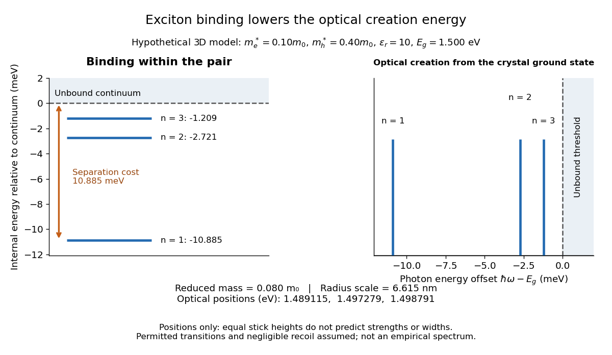
For example, the lowest internal bound state in this hypothetical model costs $1.489115\mathrm{eV}$ to create optically, yet needs only $0.010885\mathrm{eV}$ more to dissociate. The large creation energy and the small exciton binding energy answer different physical questions. An electron-hole recombination event can instead release excitation energy by photon emission or to other degrees of freedom; an emitted photon need not reproduce the original absorption energy if relaxation intervened.

A Frenkel exciton is an exciton whose internal excitation is concentrated on the scale of one molecule or unit cell. The local excitation can transfer between sites; localized internal structure does not require an immobile center of mass. The large-radius Wannier-Mott exciton approximation cannot simply be extrapolated to this limit.^[ref]

A Wannier-Mott exciton has an internal wave function extending over many unit cells. Its simplest model assumes a three-dimensional bulk crystal, approximately parabolic valence band and conduction band, positive isotropic scalar effective masses $m_e^{\ast },m_h^{\ast }$, a constant scalar relative permittivity ${ϵ}_r$, and a dilute pair population. Replace microscopic crystal forces by those effective masses and dielectric screening, and neglect exchange corrections and coupling to phonons. These assumptions must hold on the spatial and energy scales of the particular exciton.

With relative coordinate $\mathbf{r}={\mathbf{r}}_e-{\mathbf{r}}_h$, the internal Hamiltonian operator is the three-dimensional hydrogen atom problem with a reduced mass and a screened Coulomb potential:Here $e$ is the elementary charge, ${ϵ}_0$ the vacuum permittivity, and $\hslash$ the reduced Planck constant. The internal energy eigenvalues, radius scale, and exciton binding energies areThe principal quantum number is $n=1,2,\dots$. This reduction and these scales are derived in Excitons in Semiconductor Quantum Dots by Matjaž Humar (§3, printed pp. 5–6, equations (13)–(26)).

To check the scales by dimensional analysis, write $C=e^2/(4\pi {ϵ}_0{ϵ}_r)$, which has units of energy times length. Then $a_B^{\ast }={\hslash }^2/(\mu C)$ is a length and $R^{\ast }=\mu C^2/(2{\hslash }^2)$ is an energy. Rescaling $r=a_B^{\ast }\rho$ makes $H_{\mathrm{rel}}/R^{\ast }=-{\nabla }_{\rho }^2-2/\rho$, the dimensionless hydrogen atom operator. The Bohr radius $a_B^{\ast }$ is a wave function scale, not the radius of a classical orbit; for this model's lowest internal bound state, the mean separation is $3a_B^{\ast }/2$.

For the diagrams' hypothetical inputs $m_e^{\ast }=0.10m_0$, $m_h^{\ast }=0.40m_0$, ${ϵ}_r=10$ and $E_g=1.500\mathrm{eV}$, where $m_0$ is the free electron mass, independent substitution gives $\mu =0.080m_0$, $a_B^{\ast }\simeq 6.615\mathrm{nm}$ and $R^{\ast }\simeq 10.885\mathrm{meV}$. Here electronvolts express energy. The exciton binding energies for $n=1,2,3$ are approximately $10.885$, $2.721$ and $1.209\mathrm{meV}$. These are model calculations, not measured material parameters. The large-radius approximation additionally requires $a_B^{\ast }$ to be much larger than the crystal's unit cell length scale. In a thin layer, with anisotropic effective masses, or with spatially varying dielectric screening, this three-dimensional formula is not generally valid.