
Exciton binding energy Created 2026-10-14 Updated 2026-10-20
The exciton binding energy is the positive energy needed to separate a bound electron and electron hole into the relevant unbound scattering states. Compare the exciton energy with the continuum threshold at the same total crystal momentum and for the same energy bands. The negative internal energy eigenvalue and the positive separation cost are different sign conventions for related quantities. An exciton may move freely through a perfect crystal while remaining internally bound: “free exciton” does not mean an unbound pair.
Franck-Hertz experiment Created 2026-10-14 Updated 2026-10-20
The Franck-Hertz experiment connects a reproducible loss of electron kinetic energy with excitation of a chemical atom. The original mercury-vapor experiments were performed during 1912–1914 while investigating ionization; they were not designed as a test of the Bohr model. Their later interpretation distinguished internal excitation from removal of an electron. [ref]
https://labs.physik.kit.edu/prakt-klass-physik-manuals/P2/Franck_Hertz_Versuch/. KIT physics laboratory, H23 Franck-Hertz-Versuch, Motivation
.In a modern mercury tube, a heated cathode emits electrons and a positive perforated grid accelerates them through Hg vapor. A collector slightly below the grid's electric potential rejects slow electrons. The oven controls vapor density and hence the mean free path. Keep heating and retarding settings fixed, sweep the accelerating electric potential difference , and record collector electric current . These measured quantities indirectly probe atomic excitation. [ref]
https://physlab.org/wp-content/uploads/2016/03/Franck_exp_v12015.pdf. Shah, Alam and Anwar, Electron energy loss investigated through the Franck-Hertz Experiment, sections 3–4
.The curve shows repeated current minima, typically about apart. In the collision model, an electron gains approximately of kinetic energy, with the positive elementary charge. An inelastic collision transfers about to internal excitation. Near the grid, this can prevent the electron crossing the retarding region, lowering collected electric current. Further acceleration restores collection; repeated excitation losses produce further minima. These represent multiple collisions, rather than equally spaced atomic energy eigenvalues. Contact potentials shift the first minimum, so compare several successive spacings instead of identifying the first dip's voltage with the excitation cost. [ref]
https://physlab.org/wp-content/uploads/2016/03/Franck_exp_v12015.pdf. Shah, Alam and Anwar, sections 3.1–4 and Figure 3
.The optical comparison supplies a second observable: mercury radiation at a wavelength near was detected through a window in the tube. Its inferred photon energy agrees with the characteristic collision loss, with the speed of light. This agreement supports the interpretation as a transition between internal atomic energies. It does not make the collector trace a complete spectrum. In particular, the lowest excited mercury level, labeled , is metastable because an electric-dipole selection rule forbids its direct transition to the ground state; the nearby level emits the quoted ultraviolet line. Collision excitation and optical detection therefore have different sensitivities to the available excited states. [ref]
https://ocw.mit.edu/courses/8-13-14-experimental-physics-i-ii-junior-lab-fall-2016-spring-2017/afdfff9f8bbe067239af19c8b178a764_MIT8_13-14F16-S17exp7.pdf. MIT Junior Lab, The Franck-Hertz Experiment, section VI and the discussion following Figure 6
.Initial electron kinetic energy spread and varying collision positions broaden real minima. Repeat traces at different retarding settings and oven temperatures to distinguish excitation from collection effects. This probes a discrete energy-transfer channel, rather than every energy eigenspace, its dimension, or an absolute ground-state energy. [ref].
James Franck and Gustav Ludwig Hertz presented their paper on 24 April 1914. Its heated platinum wire sat inside a cylindrical platinum mesh, with a collector 1–2 mm beyond it. A heated bath and pumping prepared the vapor; guard rings suppressed leakage. They differentiated retarding-electric current scans to study outgoing energies.[ref]
Their 1925 Nobel Prize preceded their lectures of 11 December 1926. James Franck described choosing pressure for many collisions before the mesh but few afterward.[ref]
Transformations of Kinetic Energy of Free Electrons into Excitation Energy of Atoms by Impacts by James Franck. Nobel Lectures, Physics 1922–1941; pp. 98, 100–101
Gustav Ludwig Hertz explained how a field-free collision region narrowed excitation thresholds.[ref]The Results of the Electron-Impact Tests in the Light of Bohr’s Theory of Atoms by Gustav Ludwig Hertz. Nobel Lectures, Physics 1922–1941; pp. 112, 119–120
Frequency-dependent payoff 2026-10-14
A frequency-dependent payoff is an expected payoff depending on the population composition . Under random pairwise encounters with a fixed payoff matrix it is the linear function . The relative advantage can change sign as opponents become more or less common. The replicator equation converts this feedback into changes of frequency; nonlinear frequency-dependent payoffs allow interactions not represented by a fixed pairwise table.
Replicator equation Created 2026-10-14 Updated 2026-10-20
The replicator equation says that a strategy grows in frequency when its expected payoff exceeds the population's current mean payoff. It is an ordinary differential equation for a composition, rather than for total population size. The subtraction of the mean is what makes relative success matter: even a type growing in absolute number can shrink as a fraction if other types grow faster.
Let be the frequency of pure strategy , with available pure strategies andIn a symmetric bimatrix game, let the payoff matrix have entry equal to the payoff to strategy against . The other player's payoff in that encounter is : symmetry between player roles does not require . Uniform random encounters give the expected payoffs and their population meanAfter choosing the time unit so that the growth-rate scale is one, the continuous-time replicator equation isHere a payoff is measured on a scale proportional to net growth per unit time, not merely as an arbitrary preference ranking. More generally one can specify locally Lipschitz frequency-dependent payoffs directly; the same equation with then defines a unique frequency trajectory. The linear pairwise model and its reproductive interpretation are given in Taylor and Jonker (1978), sections 2–3; the formulas here also follow by the following direct normalization.
Suppose the number of type obeys , where the baseline is identical for all types. Set and . The quotient rule givesThus the common baseline cancels. Adding the same constant to every entry of leaves the replicator equation unchanged; multiplying by a positive constant changes only the speed along trajectories. The same payoff matrix can therefore describe frequency evolution at different growth-rate baselines and time scales.
The probability simplex is invariant in forward time. On ,Normalization alone would not exclude negative frequencies. Nonnegativity follows as well: along a solution,An absent type remains absent, and a positive frequency remains positive at every finite time. For the fixed payoff matrix model, bounded rates on the compact probability simplex give global forward solutions. Frequencies can still tend to zero as . Each face is invariant, so this model has no spontaneous introduction of new pure strategies; mutation or outside introductions would require additional terms. For two present types the logarithm of their frequency ratio satisfies , directly expressing the accumulated payoff advantage.
For two pure strategies, write the composition as , where is the frequency of strategy 1, and letTheir payoff difference and the resulting scalar ordinary differential equation areIn the interior , the sign of the payoff difference determines the direction of motion. The endpoints are always equilibrium points, and an additional interior equilibrium point exists precisely when the affine payoff difference has a zero strictly between them. At a simple interior zero , : a negative value gives asymptotic stability, a positive value gives instability. At the endpoints and , with stability understood relative to . A zero derivative requires examining the actual flow rather than this strict sign test.
For an original coordination game, imagine two conventions that reward matching, with convention 1 giving the larger matching reward. ChooseThe crossing is . Below it, convention 1 loses frequency; above it, convention 1 gains frequency. The endpoint equilibrium points and have one-sided asymptotic stability, while is unstable: the corresponding derivatives are and , respectively. Every initial tends to , every initial tends to , and exactly stays there. Even the convention with the larger matching reward can disappear if it starts below the threshold. This is bistability, not selection of a universally best convention.
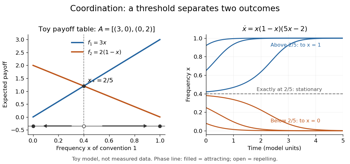
Toy coordination model: an unstable frequency threshold separates attraction to the two pure conventions
. Details. 
The compositions giving a symmetric Nash equilibrium in this coordination game are the two pure conventions and the mixed composition . Both pure conventions are evolutionarily stable strategies because a mutant convention has strictly lower payoff against the pure resident. The mixed symmetric Nash equilibrium is not an evolutionarily stable strategy: against that resident both conventions tie, but after a pure convention-1 mutant is introduced its payoff advantage is . Equal payoffs at a symmetric Nash equilibrium need not provide resistance to invasion or asymptotic stability.
For an original coexistence model, choose payoffs making each convention advantageous when sufficiently rare:Here attracts every initial composition with both types present: below it and above it. The interior derivative is , while and make both endpoints unstable to introduction of the other type. The endpoints nevertheless remain stationary if the other type is exactly absent; the attraction statement excludes those boundary initial states.
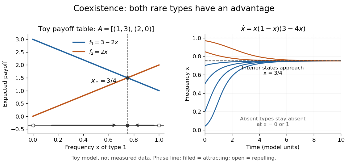
Toy coexistence model: both rare types can invade, and every interior composition approaches frequency three quarters
. Details. 
The sole symmetric Nash equilibrium in this coexistence model is . It is also an evolutionarily stable strategy. For any different mixed strategy , the first comparison in the two-condition criterion for evolutionary stability ties because . Its second comparison is strictly positive:Thus restoring frequency feedback can protect a mixture even though all present types earn equal payoffs at the mixture. Coexistence here means different individuals using different pure strategies; it does not require every individual to randomize with a mixed strategy.
Frequency evolution need not increase the mean payoff. In the coexistence example , whose maximum occurs at , whereas the attracting composition is . For , the frequency increases while . Individual payoff advantages drive the equation; maximizing collective mean payoff is a different optimization problem.
More generally, a rest point only equalizes payoffs among present types: implies . A symmetric Nash equilibrium additionally requires for every absent type. All vertices are rest points even when an absent type could invade. For finite symmetric bimatrix games, a rest point with Lyapunov stability on the full probability simplex is a symmetric Nash equilibrium; an interior trajectory that converges has a symmetric Nash equilibrium as its limit. These are conditional results, not a convergence theorem for every trajectory. See Cressman and Tao (2014), Theorem 1.
The rock paper scissors payoff matrix gives an explicit obstruction to universal convergence:Since , , and in the interior . Thus is conserved. Its maximum on the probability simplex occurs only at , the unique symmetric Nash equilibrium, so an interior trajectory starting elsewhere cannot converge to that composition. Every other interior product level is a closed curve without a rest point, giving a periodic orbit. The existence of these cycles is also discussed in Cressman and Tao (2014), Example 1. The useful lesson is to inspect the specified payoff feedback and dynamical system, rather than infer convergence from the existence of an evolutionarily stable strategy or a Nash equilibrium.
For mixed-strategy expected payoffs put and . The invasion payoff difference is exactly . Positivity for all sufficiently small positive forces by taking the limit. When , it forces . Conversely makes the difference positive for sufficiently small frequency, and makes it positive for every positive frequency. Apply this separately to every distinct mutant. This proves the equivalence with an evolutionarily stable strategy; affineness in population composition is essential to the formula.
Hawk-Dove game 2026-10-14
Hawk fights for a resource of value , while Dove retreats from Hawk and shares with another Dove. Hawk–Hawk competition incurs damage cost . The expected payoff difference between Hawk probabilities against population probability is . For positive , pure Hawk is an evolutionarily stable strategy when . At , it remains stable because a mutant loses against its own population. When , the stable mixture has Hawk probability : all first-condition payoffs tie, and its second-condition advantage is . For nonpositive resource values, pure Dove is stable if or if . At all payoffs vanish and there is no evolutionarily stable strategy.
Selection gradient 2026-10-14
For a differentiable rare-mutant invasion fitness against resident trait , the selection gradient gives the first-order growth advantage of a nearby mutant. A zero gradient is a candidate interior evolutionary singularity. Strict local uninvadability follows from negative mutant-fitness curvature; evolutionary approach additionally requires the gradient to point toward the candidate. Boundary traits require one-sided tests. A gradient alone does not prove global evolutionary stability.
Horizon-free Minkowski spacetime 2026-10-14
Every event in complete Minkowski spacetime emits a future-directed null geodesic ending on future null infinity. Therefore its black-hole region is empty and there is no intrinsic event horizon. The null edges of the Minkowski conformal compactification represent infinity, not hidden regions inside the physical spacetime. An accelerated observer can instead have an observer-dependent Rindler horizon.
Eulerian trail 2026-10-14
An Eulerian trail, also called an Eulerian path, is a trail in a graph traversing every edge exactly once. The name Eulerian path does not require a graph path: vertices may repeat. A Hamiltonian path instead visits every vertex exactly once, and may omit edges. An Eulerian trail may omit isolated vertices, so these are different coverage requirements.
For a finite undirected multigraph with at least one edge, allowing self-loops, an Eulerian trail exists exactly when the edge support of a graph is a connected graph and there are zero or two vertices of odd vertex degree. In the two-odd-vertex case they must be the two distinct endpoints; in the zero-odd-vertex case every Eulerian trail is an Euler circuit. Count a self-loop twice in the vertex degree but once in the trail, and count each parallel edge separately.[ref]
Math 530 Spring 2023, Lecture 6: Multigraphs and digraphs. pp. 1–3, Theorem 1.1.2 and the note about isolated vertices
The parity obstruction is local: each intermediate visit pairs an arriving edge with a departing edge. Only the distinct endpoints can have an unpaired incidence. The handshaking lemma, , also shows that the number of vertices with odd vertex degree is even. Sufficiency in the two-endpoint case reduces to the Euler circuit criterion: add one extra edge between the odd vertices, construct an Euler circuit, rotate its record to start with the extra edge, then delete that edge. The remaining trail has the required endpoints.
For the Seven Bridges of Königsberg multigraph, the vertex degrees at are , so no Eulerian trail exists. Remove the unique edge : the vertex degrees become , and a six-edge Eulerian trail runs from to . Label the parallel edges between and between ; label by and by . A complete record is . It revisits while using every remaining edge once.
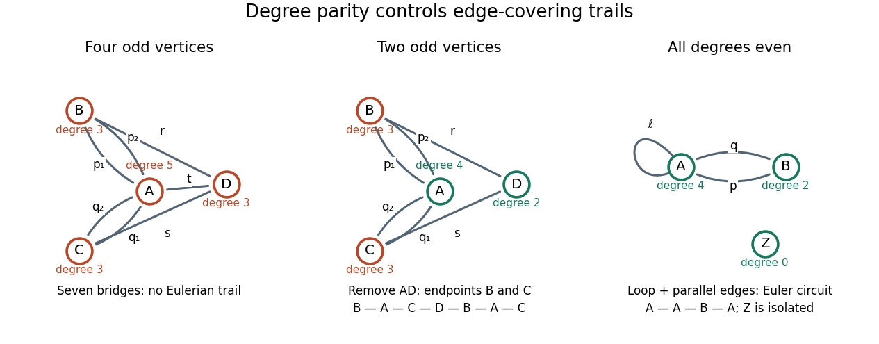
Four odd vertex degrees forbid an Eulerian trail; two allow distinct endpoints; zero allow an Euler circuit
. Details. 
Seven Bridges of Königsberg 2026-10-14
Model the four land regions by vertices and the seven bridges by distinct edges: two , two , and one each of . Their vertex degrees are . Leonhard Euler's paper records these connections in §6 and the obstruction in §9; §20 states the zero-or-two odd-region rule. Four odd vertex degrees exclude an Eulerian trail, even if returning to the starting vertex is optional.[ref]
Edge support of a graph 2026-10-14
For a finite undirected multigraph , its edge support of a graph is the subgraph with . It removes exactly the isolated vertices, retaining every edge, including self-loops and parallel edges. When , connectivity of this subgraph is the relevant condition for an Eulerian trail or Euler circuit.
Inviscid core Created 2026-10-14 Updated 2026-11-05
An inviscid core is the part of a high-Reynolds number flow outside thin wall or shear layers, where viscosity is negligible at the retained asymptotic order. It obeys the Euler equations for an inviscid fluid. Its tangential velocity need not satisfy no slip at a material wall; adjoining viscous boundary layers supply that condition and can influence the core through displacement and pressure matching.
Polymerization-driven cantilever postbuckling Created 2026-10-14 Updated 2026-11-05
A clamped filament touching a laterally sliding, moment-free wall has fixed projected gap . For an inextensible small-amplitude elastica, parameterize its tip angle by . Then and , where are complete elliptic integrals. Their small- expansions give the displayed decrease of wall force with excess contour length. It concerns the weakly buckled branch, before overhang or additional wall contact changes the boundary conditions.
Planar domain 2026-10-14
A connected open subset of the Euclidean plane. For a bounded polygonal example, the Dirichlet Laplacian is the self-adjoint operator associated with the Dirichlet energy on ; its eigenfunctions are smooth in the interior but need not be smooth at reentrant boundary corners.
Complex lattice 2026-10-14
A complex lattice is a discrete rank-two subgroup of the complex plane, generated by two real-linearly independent periods. An oriented basis can be chosen with . Scaling by then gives for a point in the complex upper half-plane.
Lenstra-Lenstra-Lovász lattice basis reduction algorithm Created 2026-10-14 Updated 2026-10-20
For an integer basis of a Euclidean lattice, the algorithm uses integer column operations and swaps to obtain a size-reduced basis with Gram-Schmidt coefficients and the condition . It preserves the lattice and exposes short vectors and near-relations. It is useful for improving proven Diophantine bounds by encoding scaled logarithms in integer coordinates. A certified lower bound for every nonzero lattice vector is : in a nonzero integer linear combination, project onto the last nonzero Gram-Schmidt direction. Better-reduced bases improve this lower bound. Rounding and logarithm errors must still be bounded before turning it into a certified lower bound for a logarithmic form.
Long division 2026-10-14
Repeated division with remainder that determines successive digits of a quotient. To generate the fractional digits in base , multiply the current remainder by , divide by the denominator, and keep the resulting remainder for the next step.
Remainder 2026-10-14
Etendue bench measurement 2026-10-14
A proposed optical bench test uses a steady illuminated diffuse patch, a relay made from two optical lens elements, interchangeable centred circular stops, and a calibrated optical power meter large enough to collect the whole output bundle. Start with small cone angles so an ordinary relay approximates the area-angle tradeoff. Measure the patch's image diameter and the accepted angular extent at both conjugate planes; the transverse magnification gives the spatial scale, but does not by itself measure etendue.
Map the local radiance with a baffled photodiode on translation and rotation stages, using two small aligned holes to select a narrow known solid angle. Keep the sampled position fixed while scanning direction, calibrate the sampling footprint and angular response, and repeat at several positions. Numerically integrate over the occupied samples, and integrate to predict the collected radiant flux. This checks the filled-cone assumption instead of inferring it from two outer dimensions.
Compare the relay without a stop and with a stop of times the illuminated diameter in the same plane. The uniform-bundle prediction is a radiant flux ratio of , with unchanged local radiance in the surviving samples. Cover the input for a dark reading, monitor source drift, repeat the open-stop reading, check detector linearity with calibrated optical attenuators, and enlarge the collecting detector or scan it to check for missed light rays. Lens losses, angular response, illumination gradients, alignment errors and diffraction can spoil the ideal prediction; their effects must be measured separately. This is a procedure to try, with predicted readouts, not purported experimental data.
Optical concentrator Created 2026-10-14 Updated 2026-11-05
An optical concentrator redirects light from an entrance area to a smaller receiver area . Its geometric concentration ratio is . Specify the admitted angular distribution and losses before interpreting as an irradiance gain: if a fraction of incident radiant flux reaches the receiver, the ratio of mean receiver to mean entrance irradiance is .
There are unlisted articles, also show them or only show them.