Spectral luminosity is energy radiated per unit time per unit frequency. Its frequency integral is the total luminosity. For an isotropic source at small distance , neglecting attenuation and cosmological effects, the spectral flux density is .
The luminosity per unit spatial volume. For a spherical source, its enclosed luminosity is , and its projected surface brightness is .
Fixed-quota harvesting of Lotka-Volterra populations by  Codex 0 Created 2026-10-14 Updated 2026-11-05
In logarithmic prey/predator coordinates, the Lotka-Volterra predator-prey model has divergence zero. Removing a fixed prey quota changes to and expands logarithmic area by . Thus a periodic annually harvested orbit has an expanding return map determinant and cannot be asymptotically stable. A continuous-quota approximation gives a coexistence equilibrium with positive Jacobian matrix trace , unlike proportional harvesting, which only changes the prey growth parameter in this idealized model.
An annual pulse-breeding predator-prey model combines continuous predation and mortality between short reproduction episodes with an annual difference equation. If surviving predators produce offspring in proportion to prey surviving the year, retained adults give the displayed map. Here combines prey reproduction and natural survival, is predator survival, and integrates predation over declining predator abundance. The positive annual equilibrium is , for and .
The velocity-addition formula translates a particle's velocity between two specified inertial frames. Let move at signed velocity along the -axis of , with parallel axes and , where is the speed of light. Define and for the same particle's world line, using position and time measured within the corresponding inertial frame. With Lorentz factor , the forward Lorentz boost gives
For collinear motion, write and . The inverse velocity-addition formula isThis is the composition of the particle's velocity in and that frame's velocity relative to . The velocities must belong to this same chain of reference frames, with directions specified. Two arbitrary quoted speeds cannot be inserted blindly. Each velocity measurement uses distances and clocks in a single inertial frame, with Einstein synchronisation for separated clocks.
For example, let and let the particle travel at in . Its velocity in isThe Galilean transformation would instead give , which fails here. For light moving along the positive axis, gives ; similarly gives . Negative directions also work for massive particles: at , gives , while gives . Thus “addition” means composition of signed velocities, rather than addition of their magnitudes.
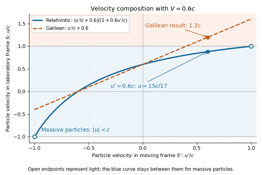

A short derivation differentiates the Lorentz transformation: and . Dividing these differentials gives the longitudinal velocity-addition formula. The transverse formulas use and , but the same transformed time denominator; omitting it would ignore the relativity of simultaneity. Replacing by gives the inverse. When both relative and particle velocities are small compared with the speed of light, the denominator is close to one and the nonrelativistic limit recovers the Galilean transformation.
The formula lets us compare particle motion in a moving apparatus and a laboratory without losing the invariant speed of light. Einstein's 1905 paper derives the coordinate change in §3 and the composition of velocities in §5, including the collinear formula, its light-speed case, and composition of parallel transformations. [ref]
https://www.fourmilab.ch/etexts/einstein/specrel/www/. Albert Einstein, On the Electrodynamics of Moving Bodies (1905), §§3 and 5; English translation by W. Perrett and G. B. Jeffery, electronic edition by John Walker
. The rapidity parametrization makes the collinear composition particularly simple.An orthonormal coframe in spacetime can be rotated by a position-dependent Lorentz matrix without changing the spacetime metric tensor. Its spin connection transforms as . A spinor field transforms through a chosen spin lift , not through the vector matrix . With , an infinitesimal parameter gives , where . Consistent global transition lifts require a spin structure; a spatial rotation lifts to minus the identity on spinors.
Lithium-7 has three protons and four neutrons. In Big Bang nucleosynthesis it can form directly or through beryllium-7, which later undergoes electron capture. Competition between direct lithium production, lithium destruction and beryllium production produces a valley in the primordial lithium abundance versus baryon-to-photon ratio. Its measured stellar surface abundance need not equal its birth abundance because stellar transport and nuclear burning can remove lithium.
A physiologist who developed the concept of homeostasis: interacting physiological processes maintain relatively stable internal conditions despite disturbances. In his account, stability is an actively maintained outcome rather than absence of ongoing change.[ref]
Homeostasis (excerpt from The Wisdom of the Body). 1932, opening discussion of resistance to changes

Portrait of Walter Bradford Cannon
. Wellcome Library, London / Wellcome Collection. CC BY 4.0, via Wikimedia Commons. Source.
A membrane leaflet is one of the two layers forming a lipid bilayer. In a phospholipid-based cell membrane, the hydrophilic regions face the adjacent water, and the hydrophobic regions face the interior shared by the two membrane leaflets.
For two segregating biallelic loci, encode the allele on a random biological population haplotype by indicator variables . Their covariance is the linkage disequilibrium coefficient . The squared correlation is , between zero and one. It measures how well one marker predicts the other and is undefined if either marker is monomorphic.
// Target: biology.bigb
Genetic recombination erodes linkage disequilibrium by reshuffling alleles between haplotypes, while preserving marginal allele frequencies in the idealized model. Let denote the haplotype frequency in the gamete pool of generation , let denote its marginal allele frequencies, and let be the constant recombination fraction between two autosomal genetic loci. Assume random mating within one population, nonoverlapping generations, fair Mendelian segregation, equal reciprocal gamete production, the same in both sexes, and a deterministic population large enough to neglect genetic drift. Exclude natural selection, mutation and gene flow. ThenHere and remain constant: recombining changes which alleles occur together, not their total numbers. The other haplotype frequencies change by for and for . Consequently the joint probability distribution stays within its allowed bounds and approaches the product of its marginal distributions when .
For the original positive example , a recombination fraction gives and . The negative example has exactly the opposite sequence: genetic recombination reduces the magnitude without reversing the sign. With , the initial linkage disequilibrium persists in this model; even independent assortment at only halves each generation. A population association does not vanish after one generation merely because the genetic loci are unlinked.
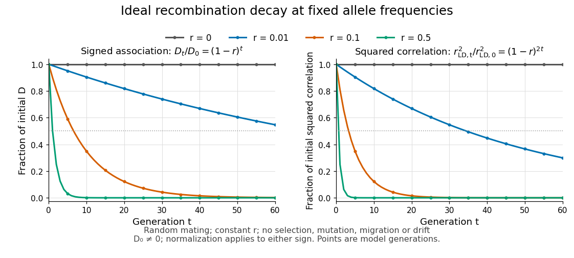
Idealized linkage-disequilibrium decay under recombination at four recombination fractions, with faster decay of squared allelic correlation when marginal allele frequencies remain fixed
. Details. 
The geometric sequence gives a generation scale: for , the continuous interpolation reaches at . Actual generations are integers; the first at or below half is . For small , . Because the denominator of allelic correlation stays fixed, ; its decay is faster than the magnitude of .
A short derivation uses random mating to assign frequency to the double heterozygote and to . Relative to , each loses or gains an gamete fraction , respectively. Their net contribution is . The other genotypes produce no net change in , proving the recurrence and, by iteration, its solution.
This temporal model does not identify elapsed generations from physical separation alone. The recombination fraction depends on genetic recombination, including recombination hotspots, while population stratification, natural selection, gene flow or genetic drift can create or maintain linkage disequilibrium. Repeated sampling across time would also require accounting for sample size and haplotype estimation. A cross-sectional plot of association against distance between genetic loci is therefore a different observation from the idealized trajectory plotted here.
For positive linkage disequilibrium , take ; for negative , take and retain its negative sign in . Thus . Its magnitude measures the fraction of the largest disequilibrium possible at the specified allele frequencies. High need not imply high allelic correlation, so it does not alone guarantee good marker prediction.
For two genetic loci with two alleles each, linkage equilibrium is independence of their states on sampled haplotypes. It concerns association between genetic loci; Hardy-Weinberg equilibrium concerns pairing of alleles into diploid genotypes.
The Newtonian limit of general relativity describes slowly moving matter in a weak, approximately static gravitational field. With metric signature and , identify the Newtonian gravitational potential byNeglecting time derivatives and terms of higher order in particle velocity divided by the speed of light, the spatial geodesic equation becomesThis recovers Newtonian gravitational acceleration rather than merely matching a metric coefficient.
For nonrelativistic matter, dominates the stress-energy tensor. With negligible anisotropic stress, the weak-field Einstein tensor gives . Matching to the Poisson equationtherefore fixes . Setting gives the commonly written and . Relativistic pressure, rapid time variation or strong gravitational fields requires terms omitted in this limit.
For a static spherical point source, the weak-field solution in isotropic radius has and spatial metric . The isotropic-to-areal weak-field radius change gives the displayed metric with . Its validity requires . Treating it as an exact metric near can turn omitted terms into large corrections; it does not establish horizons or strong-field photon dynamics.
For static scalar perturbations with no mixed time-space or spatial shear terms, the displayed metric tensor uses signature . With the reversed convention in curvature-sign convention in Killing derivative identities, its first-order Einstein tensor is , , and . These follow by substituting the metric into the first-order Christoffel symbols and Ricci tensor, discarding products of perturbations. A static source with the dust stress-energy tensor obeys and the decaying spatial equation makes . For a point mass the Newtonian potential of a point mass gives , . The spatial potential is necessary to determine light propagation; a time potential alone is insufficient.
For signature , decompose a metric perturbation into , and , where the spatial vectors are divergence-free and is a transverse-traceless tensor. Under a passive coordinate shift , , with , the changes are , , , , , and . The displayed combinations and are therefore gauge invariant. The decomposition is unique after appropriate spatial decay or mode restrictions; homogeneous and boundary modes require separate conventions.
An inhomogeneous linear recurrence has a prescribed forcing sequence rather than zero on the right. The difference of two solutions satisfies the associated homogeneous linear recurrence relation, so every solution is a particular solution plus a homogeneous solution.
For two solutions of the linear recurrence relation , their discrete Wronskian obeys . Substitute the recurrence into : the terms cancel and the remaining expression is . Iteration gives , including when some vanish. A nonzero discrete Wronskian proves linear independence of the two solutions.
For , and terminal cost plus running cost , the displayed change of state gives . A quadratic value function has coefficient and additive noise cost . Minimizing its Hamilton-Jacobi-Bellman equation gives the displayed control. The gain is unchanged if the additive noise is removed, illustrating certainty equivalence.
There are unlisted articles, also show them or only show them.