
Consider a stipulated dilute collection of independent two-level systems, each with longitudinal magnetic moment , , and energy . The prescribed vacuum/applied magnetic flux density is . Ignore interactions, orbital magnetic response, and the small sample-field correction. This is the magnetic version of the existing independent spin-one-half two-level system, with alignment probabilities rather than an interacting Curie–Weiss model.
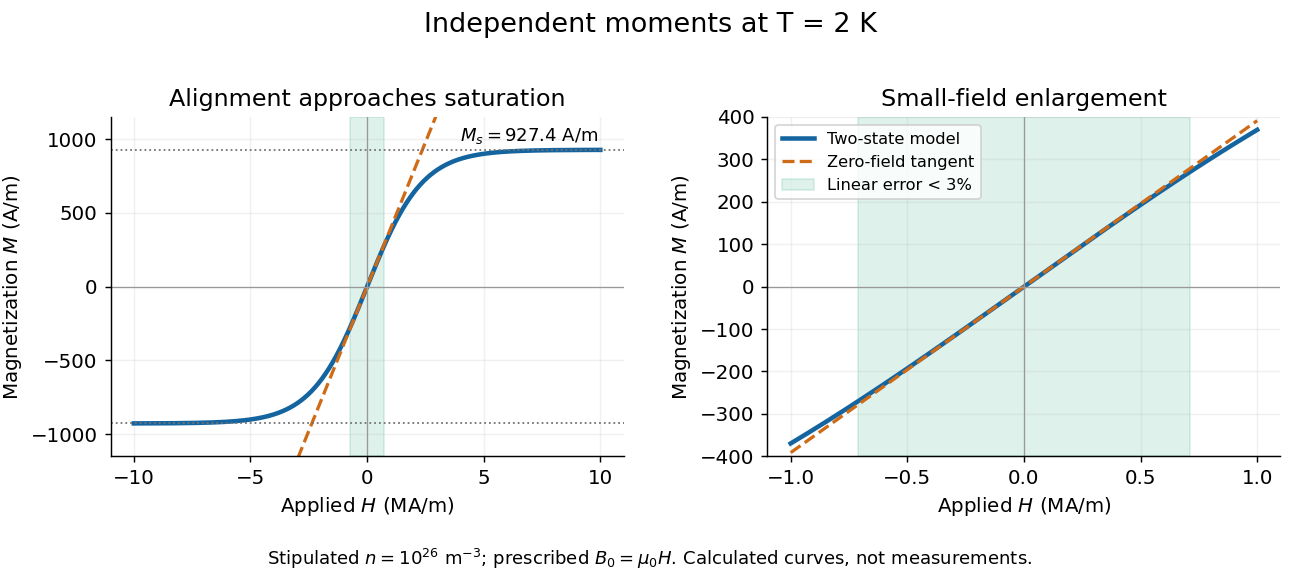
For temperature , the canonical ensemble gives the one-moment partition function , with . Taking the expected value over its two Boltzmann weights givesHere is the number density, the Boltzmann constant, and the hyperbolic tangent. For , its small-argument expansion of the hyperbolic tangent gives , a Curie's law response in the applied- convention. For large , approaches the saturation magnetization with sign set by the field, and its differential magnetic susceptibility falls towards zero.
Both plots use stipulated , , , and . The moment is approximately one Bohr magneton; the chosen vacuum permeability is a rounded model input. At , and . The linear approximation overestimates by less than for , corresponding to or . These parameters keep the modeled response weak; neglected magnetic feedback is of relative order , rather than an explanation of a material's ordered phase.

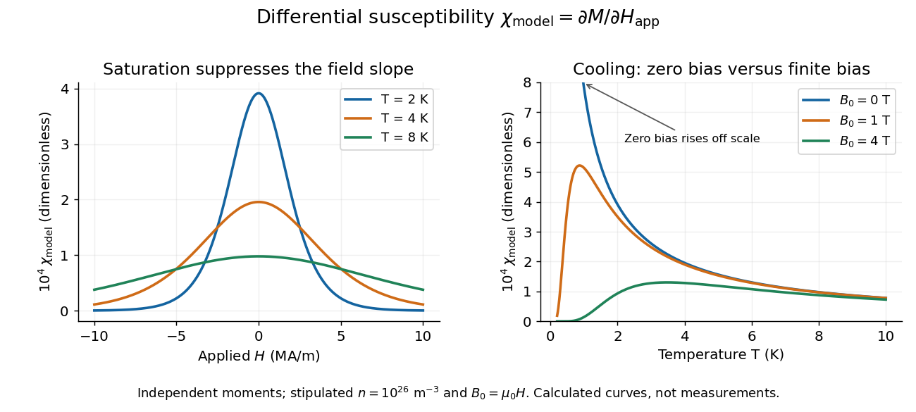
Bias-field and temperature dependence of the independent-moment differential magnetic susceptibility
. Original calculation using the same stipulated moments and number density. The left panel compares field sweeps at , and . The right panel compares temperature sweeps at prescribed , and . The zero-field slope follows Curie's law; cooling at fixed nonzero field eventually suppresses the slope through saturation magnetization. Details.
At , cooling increases the zero-field slope as . At fixed , cooling instead gives : a saturated moment can hardly change further. The order of the zero-field and zero-temperature limits matters. This independent model has no finite-temperature collective phase transition; the diverging zero-field slope alone does not establish one.
The demagnetizing field is the contribution to magnetic field intensity produced by the sample's own magnetization. Inside a uniformly magnetized ellipsoid, it is uniform and has the form ; the demagnetizing factor along a principal axis gives its longitudinal component. These conditions make the scalar correction in field conventions for magnetic susceptibility useful.
A cylinder generally has spatially varying magnetization and demagnetizing field. A volume-sensitive instrument and a short central pickup coil consequently need different effective corrections: one averages over the sample, while the other samples central flux. A shape factor copied from an ellipsoid is not an exact correction for every cylinder, especially with nonlinear response or hysteresis. [ref]
Demagnetizing Factors. R. B. Goldfarb, Demagnetizing Factors, printed p. 104, §2 opening paragraphs: magnetometric versus fluxmetric sensing, nonuniform cylindrical fields and susceptibility-dependent factors
In vacuum, magnetization is zero and magnetic flux density obeys . The applied quantities and mean the field of the external sources at the sample position with the sample absent. The internal magnetic field intensity includes the sample's demagnetizing field; its internal magnetic flux density additionally includes . A field quoted in the tesla is a quantity, even when an instrument informally calls it “”.
For a uniformly magnetized ellipsoid, along a principal axis with demagnetizing factor in the International System of Units,For a sphere, . The axial value approaches zero in the long slender ellipsoid limit and the normal value approaches one in the thin flat ellipsoid limit. Thus a stipulated intrinsic volume magnetic susceptibility would yield apparent values in a sphere and approximately in a long axial sample. These are calculated geometry effects, not measured material values. For fixed , implicit differentiation gives the same conversion for local differential magnetic susceptibility, .
A magnetic susceptibility tensor maps a small change of internal magnetic field intensity to a change of magnetization:This tensor reduces to for isotropy. With anisotropy, even a linear response need not point along the applied magnetic field intensity. As a stipulated example, sends to . State the axes and bias field when reporting its components. A constant tensor describes linear response; in a nonlinear material it is the Jacobian matrix of the response at the chosen operating point.
Differential magnetic susceptibility is the local slope at a specified bias magnetic field intensity, holding temperature and other stated constraints fixed. It equals volume magnetic susceptibility only for a linear response through the origin. For example, has , but , where . At these are about and times their common zero-field slope. A finite sweep chord is another quantity, not automatically this derivative.
If the differentiated field is instead the internal magnetic flux density, the longitudinal chain rule applied to givesThis differs from the vacuum/applied- conversion in volume magnetic susceptibility. It assumes a differentiable single branch with locally invertible .
Volume magnetic susceptibility is the dimensionless ratio of longitudinal magnetization to internal magnetic field intensity in a linear regime through the origin. Positive response gives paramagnetism. Always distinguish magnetization from total magnetic moment : dividing by volume changes the normalization. Mass-normalized and mole-normalized values likewise require the mass density or the volume per amount of substance before comparison with .
In the existing Pauli paramagnetism formula, denotes total magnetic moment, and is the total spin-summed density of states. Relabel that response asHere is the Bohr magneton. If its is a prescribed vacuum/applied magnetic flux density , the dimensionless apparent slope is . It agrees approximately with intrinsic only when the demagnetizing field correction and magnetic feedback are negligible. The existing Curie's law formula also uses a total-magnetic moment, -derivative convention; its counts moments rather than giving a number density.
Curie's law is the inverse-temperature magnetic response of independent magnetic moments in the weak-polarization regime. Let each moment have angular momentum quantum number , Landé g-factor , and magnetic projection , where . Its Zeeman energy is . At zero field the projections are equally likely, so and . Differentiating their canonical partition function gives the total-moment response of independent moments,For a dilute weakly magnetized sample with number density and , the dimensionless SI volume magnetic susceptibility is insteadThese conventions differ by volume, field and factors. A fixed nonzero field eventually saturates the moments as temperature falls, so the linear Curie's law regime requires .[ref]
3 Quantum Gases. magnetic response and Curie's law; Tong defines susceptibility using total moment differentiated with respect to B
The London equations relate the superconducting electric current to the electromagnetic field: and . In a gauge with constant condensate phase the second follows from ; it implies exponential magnetic field screening.
Compactifying M-theory on a circle gives type IIA superstring theory. The circle radius sets its coupling. Multiplying M2-brane and M5-brane tensions by the circle circumference gives the fundamental string and D4-brane tensions, while unwrapped objects give D2-branes and NS5-branes. Momentum and a Kaluza-Klein monopole supply D0-brane and D6-brane charges. The circle dictionary and worldvolume reductions are developed in Four Lectures on M-theory.
M-theory on a two-torus and type IIB superstring theory on a circle describe the same nine-dimensional physics. Torus shape supplies the axion-dilaton; torus area supplies the circle-radius modulus after matching metrics. An M2-brane on a one-cycle gives a (p,q) string; an M5-brane on the whole torus gives a D3-brane. Matching brane charges and tensions establishes the dictionary in The Power of M Theory.
M-theory on a K3 surface and the heterotic string on a three-torus have matching seven-dimensional moduli and charge lattices. The K3 intersection lattice supplies twenty-two vector charges; an M5-brane wrapped on K3 becomes the heterotic fundamental string. The strong-coupling interpretation and low-energy matching are derived in section 4.7 of String Theory Dynamics in Various Dimensions.
Cytokinesis partitions the cytoplasm. Without cytokinesis, two cell nuclei can share one biological cell. [ref]
Cytokinesis makes physically separate daughter biological cells by partitioning their cytoplasm and completing their cell membrane boundaries. Mitosis divides nuclear material. These processes can overlap during M phase, but completion of one does not imply completion of the other.[ref]
The Cell Cycle. Biology 2e by Mary Ann Clark and others; §10.2, The Mitotic Phase and Cytokinesis: nuclear division versus physical daughter-cell separation
For an original compartment-counting example, consider a hypothetical diploid biological cell after two daughter cell nuclei have formed. Let be the number of chromosomes in one haploid set, and let be that set's unreplicated nuclear DNA amount, as in cell-cycle DNA content. Assume faithful mitosis, no nuclear DNA replication during the partition, and no loss of nuclear DNA; exclude mitochondrion DNA.
| Counting boundary | Before cytokinesis | After cytokinesis |
|---|---|---|
| Biological cells | 1 | 2 |
| Cell nuclei in each biological cell | 2 | 1 |
| Each cell nucleus | chromosomes, | chromosomes, |
| Nuclear DNA per biological cell | ||
| Nuclear DNA across all descendants |
The check is to follow the two existing cell nuclei: initially one boundary encloses both; finally each daughter boundary encloses one. The total remains two cell nuclei, twenty chromosomes and of nuclear DNA. Thus the amount per biological cell halves because the counting boundary changes, without any new DNA replication or change of nuclear ploidy. Doubling the number of biological cells need not double their combined material.
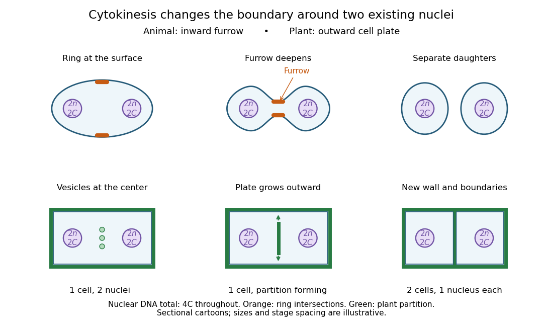

Coordinating chromosome segregation with cytoplasm partition lets descendants inherit nuclear information inside separate working compartments. Equal nuclear DNA allocations do not require equal daughter sizes or equal allocations of every organelle. The geometry of cytokinesis connects an internal allocation to the creation of two independently bounded biological cells.
Mitosis allocates copied chromosomes to daughter cell nuclei. The spindle apparatus aligns sister chromatids before separation in anaphase.
The copying has already occurred during S phase, before mitosis. Nuclear chromosome segregation and cytokinesis, the partition of the cytoplasm, are distinct processes: two daughter cell nuclei can form inside one undivided biological cell.[ref]
The Cell Cycle. Biology 2e by Mary Ann Clark and others; §10.2, Interphase and The Mitotic Phase; Figure 10.5: replication precedes nuclear division, which can occur without cytokinesis
The original cartoon follows a hypothetical diploid animal biological cell with . Its two homologous chromosome pairs are and ; upper- and lower-case letters identify homologues, not dominant and recessive alleles. In prophase and metaphase, each replicated chromosome contains two sister chromatids: four replicated chromosomes contain eight chromatids, rather than eight replicated chromosomes. The X shape depicts two associated copies, not the shape of every chromosome throughout the cell cycle.
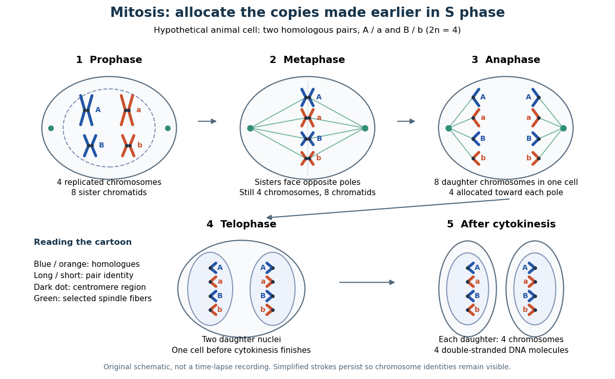

This open mitosis cartoon shows nuclear envelope breakdown and reassembly. Closed mitosis in some yeasts retains the nuclear envelope while daughter chromosomes separate inside it; the cartoon is therefore not a universal cellular architecture.[ref]
The Cell: A Molecular Approach, 2nd edition by Geoffrey M. Cooper. Chapter 8, The Nucleus during Mitosis, Dissolution of the Nuclear Envelope; Figures 8.29–8.30: open and closed mitosis
On a compact positively invariant set where , every trajectory approaches the largest invariant subset of .
For and , on either half-plane the Lyapunov function is nonnegative, has compact sublevel sets contained in that half-plane, and satisfies . The only invariant points of are and . The invariance argument therefore makes each half-plane converge to its corresponding stable focus. The stable set of the saddle at is exactly the line .
A Lyapunov functional assigns a scalar to the entire state of an evolution equation and is monotone along its trajectories. For a gradient flow , the identity follows from the variational chain rule, with boundary terms removed by periodicity or decay. A spatial density is not itself a Lyapunov functional unless all remaining coordinates are integrated or averaged.
For an open dust-only Friedmann-Lemaître-Robertson-Walker metric with zero cosmological constant and , . The present radial cosmological proper distance is , and the areal radial coordinate satisfies . Integrating with gives the displayed relation. It has near the observer and as . The luminosity distance is , not the radial cosmological proper distance.
In an Einstein-de Sitter universe normalized by , the Friedmann equation gives . Integrating the radial null geodesic gives . The luminosity distance is , yielding the displayed expression. Near the observer it is ; the limiting radial comoving distance is finite even though the luminosity distance diverges.
There are unlisted articles, also show them or only show them.