
With
MAP_PRIVATE, copy-on-write initially reuses backing page cache contents. In our model, a private store raises a protection page fault, copies the affected memory page to a private page frame, installs a writable page table entry and retries. The other memory page can remain shared. This page fault needs no storage read.In B's private file mapping, storing copies relative page 1, including its neighbor . Next, A stores through its shared file mapping. After coordination outside the mapped data, B's shared reads give , while its detached private page gives . The untouched first memory page remains backed by the file; this is not a frozen snapshot of the whole file. Neither page writeback of shared contents nor msync publishes B's private 99. To save those private contents, the application needs a separate explicit file update.
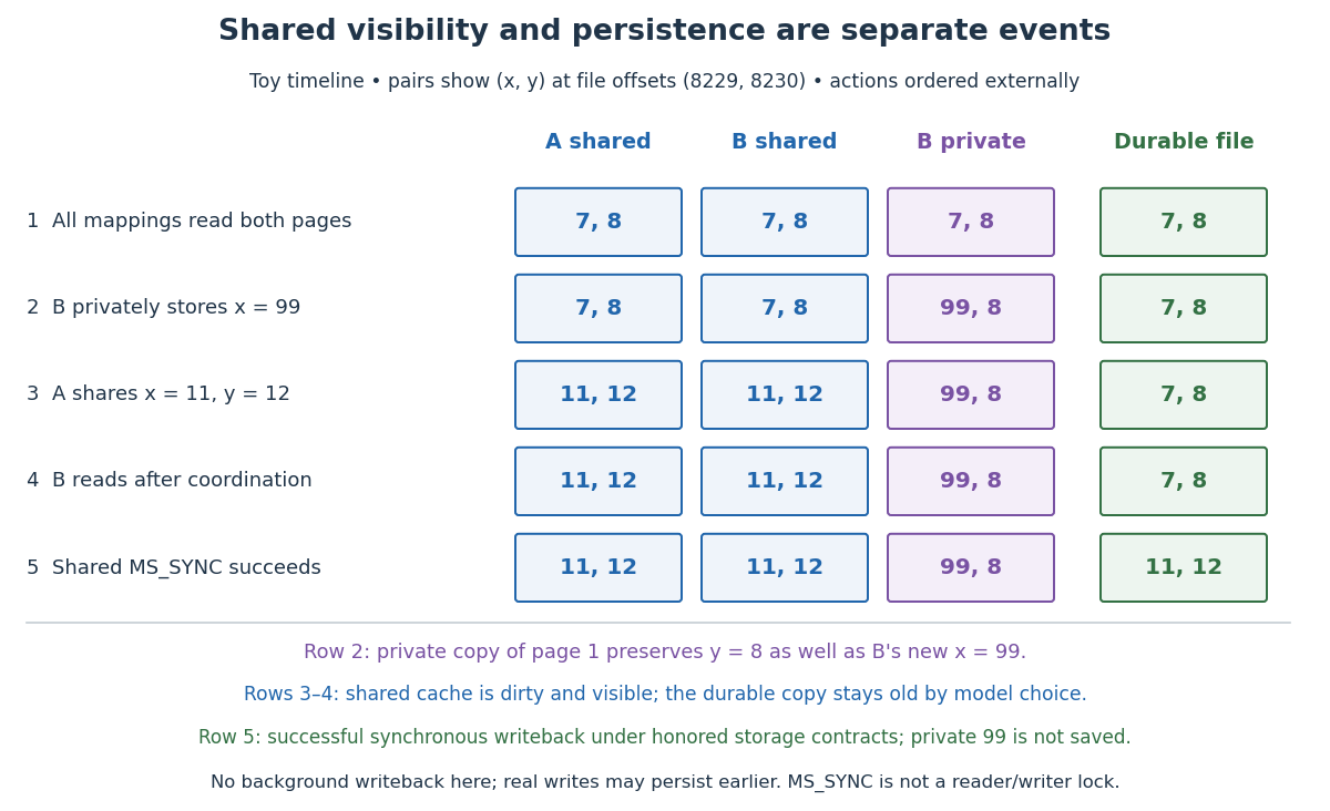
Toy shared file mapping and copy-on-write timeline: visible shared changes precede the chosen durable completion; private changes remain separate
. Details. 
Let be the memory page size, the aligned starting file offset, the mapping length and its base virtual address. A valid displacement with corresponds to file offsetHere is the relative memory page index, the floor function selects its integer part, and Euclidean division gives the within-page displacement . The backing page begins at . This identifies file contents; the page table separately selects a resident page frame and enforces permissions.
Take , and bytes in a file of at least 12288 bytes. A has a shared file mapping at . B has a shared file mapping at and a private file mapping at . These bases are illustrative chosen results, not requested fixed addresses. All three mappings cover the same two backing pages: file offsets 4096–8191 and 8192–12287. Displacement selects relative page 1, within-page displacement 37 and file offset . Thus A's
0x10001025, B's shared 0x20001025 and B's private 0x30001025 initially identify the same byte. The adjacent displacement 4134 identifies file offset 8230. Different virtual addresses can reach the same backing contents.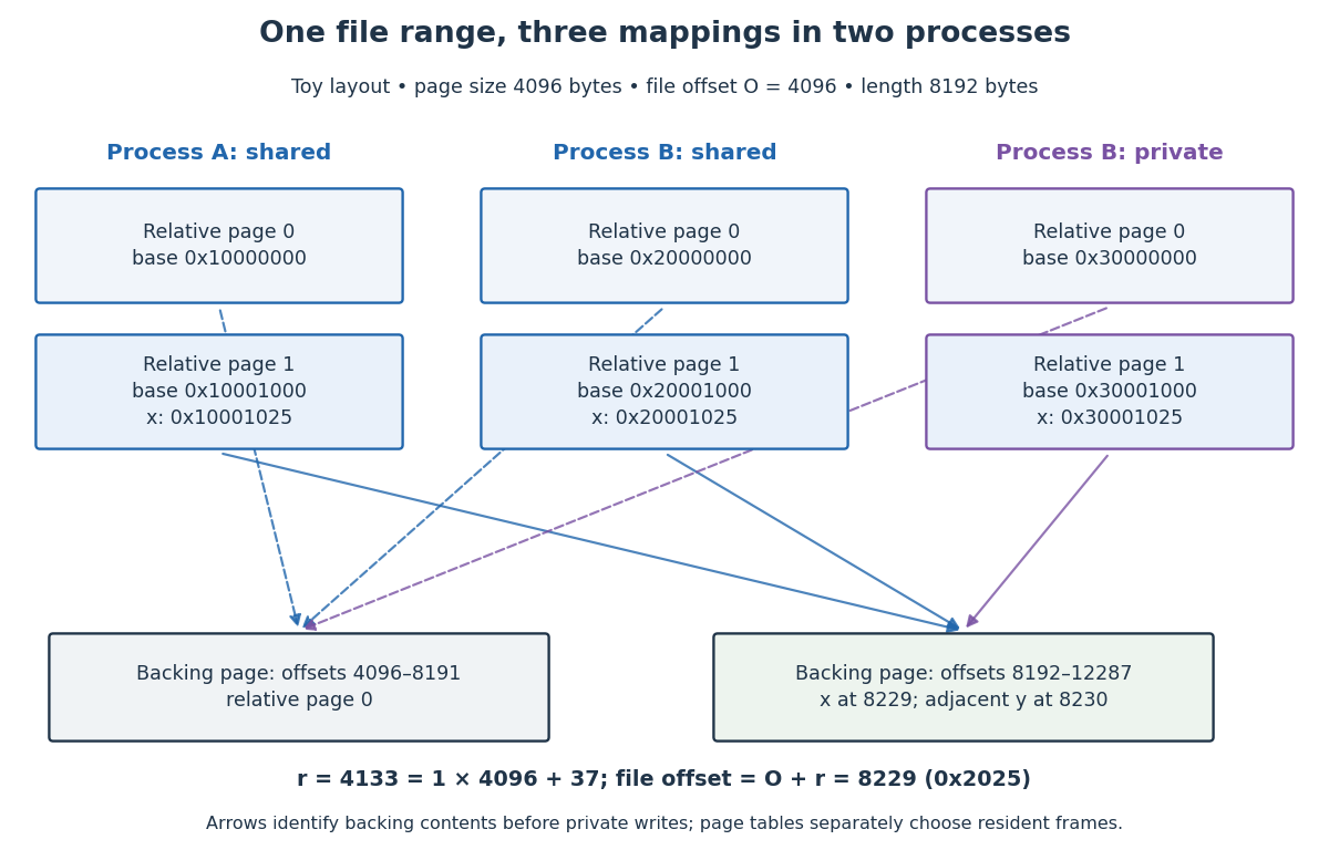
Two operating-system processes map two backing pages at different virtual addresses; displacement 4133 identifies file offset 8229
. Details. 
To access a requested file offset that is not aligned, choose and displacement . Mapping enough bytes to cover that displacement plus the requested length makes the desired data start inside the aligned mapping. Do not pass the unaligned directly as the Linux kernel
mmap offset. For example, uses and displacement 37; that one-page start differs from our two-page mapping's .The POSIX mapping interface. Ordinary Linux kernel file mappings require a positive length and an aligned file offset. A null address lets the operating-system kernel choose an aligned base; length need not be aligned. Check for
MAP_FAILED. After success the file descriptor may be closed without invalidating the mapping; munmap or process termination removes it.[ref]mmap(2) — Linux manual page. DESCRIPTION: address, length, offset and descriptor lifetime; munmap; RETURN VALUE
Mapping does not extend the backing file. Under POSIX, for an initially partial last memory page, the tail beyond the file's end is zero-filled and is not written back as file data; accesses to whole mapped memory pages beyond the end raise
SIGBUS. POSIX leaves access to portions added or removed by later resizing unspecified. Establish the required file size first and coordinate resizing with readers; a mapping's length is not proof that those bytes exist in the file.[ref]mmap — POSIX.1-2024. POSIX.1-2024, DESCRIPTION: partial end page, whole pages beyond the object, and changed file size; RATIONALE: references beyond the end do not extend the object
The Linux kernel documents a tail-cache exception: modified beyond-end bytes can survive in the page cache and appear in later mappings, although never written to the file. Do not use that tail as reliable storage.[ref]
mmap(2) — Linux manual page. BUGS: modified contents beyond the object end can remain in the page cache
The file supplying a memory-mapped file's initial contents. Its logical file offsets identify data independently of the virtual addresses chosen by different operating-system processes. Modified private file mapping contents have private storage; they are not updates waiting to be written to the backing file.
The arithmetic mean of memory access latencies. Suppose each read completes before the next begins, every cache hit costs , and every cache miss costs , with the same additional cache miss penalty . If is cache hit rate and is cache miss rate, the weighted arithmetic mean isThe common lookup cost is paid on both outcomes. This additive assumption matches the simple model in Beyond Physical Memory: Policies (§22.1, equation 22.1, pp. 1–2), where main computer memory acts as a memory cache for memory pages backed by disk; here the same accounting is applied to a toy data memory cache.
Assign synthetic values and . The twelve-read, two-slot fully associative cache example has five cache hits and seven cache misses, givingWith four cache slots, its four compulsory misses instead give . This comparison holds the timing costs fixed as capacity changes, which is a model assumption rather than a hardware promise.
If a problem supplies a total miss time , use ; adding to again would count lookup twice. Variable cache miss penalties, multiple consulted levels, or overlapping requests require a richer timing model. Real CPU work can overlap a pending read, so this arithmetic mean cannot by itself predict program speed or stall time. [ref]
A memoization cache lifetime is the interval over which retained entries are available and valid. One table per top-level request shares recursive subproblems within that request; keeping a table between requests also allows the warm and incremental examples. Clearing it loses those savings. Evicting a correct answer can preserve correctness for a terminating pure function, while forcing recomputation; changing an input without invalidating an obsolete answer can break correctness.
Specify who owns the table, when context changes invalidate it, and how long keys and results occupy computer memory. In a concrete implementation, retained references can keep arguments and answers alive until removal or clearing.[ref]
functools — Higher-order functions and operations on callable objects (Python 3.14 documentation). Python documentation, functools.lru_cache: cache_clear and retention of argument and return-value references until eviction or clearing
The memoization promise is conditional reuse of valid completed answers, not an automatic guarantee of freshness, termination or bounded computer memory.// Target: computer-science.bigb
A memoization key identifies all information that determines a reusable answer. Write for explicit arguments and for relevant context. For a function and key function , the necessary value condition isThis implication need hold only for contexts in which the entry can be reused. The condition concerns key equality, not merely equality of hash function outputs: a hash table must resolve hash collisions by comparing complete keys. Include the identity or version of the procedure if one table stores results for several procedures or changing implementations.
For an original toy example, let . Caching only by after incorrectly returns for , whose answer is . The pair is complete for this function. If is hidden in mutable configuration, either freeze that configuration for the memoization cache lifetime, include a reliable version in the key, or invalidate affected entries before reuse. A version is sufficient only if every relevant change updates it. Object identity alone is likewise insufficient for a mutable list whose contents determine the answer.
Endocytosis takes material into a biological cell by inward budding and separation of part of its cell membrane. At a chemical synapse, it helps recover membrane and proteins after synaptic vesicle exocytosis. This recovery is distinct from uptake of individual neurotransmitter molecules through membrane transport proteins.
Exocytosis releases the contents of a membrane-bounded compartment to the extracellular space by fusion with the cell membrane. Synaptic vesicle fusion is an example. Its contents are released, while its membrane becomes connected to the cell membrane; see synaptic vesicle for recovery and reuse.
Active transport moves a substance uphill in its electrochemical gradient by coupling the transfer to a downhill process. Some carrier proteins use ATP hydrolysis; others couple uphill transfer of one solute to downhill transfer of another solute, often an ion. The latter mechanism uses a stored electrochemical gradient and need not consume ATP directly at that carrier protein. Maintaining the driving electrochemical gradient still requires a source of energy. See Alberts et al.: carrier proteins and active membrane transport.
For the neutral 8:2 example, B-to-A transfer costs per mole. As an explicitly assumed bookkeeping example, suppose a tightly coupled cycle supplies a downhill free energy change of per mole of transferred solute. The total is then . This makes forward cycling energetically possible under those assumptions; it specifies neither a molecular mechanism nor a rate. Merely adding a carrier protein cannot supply the missing free energy. Conversely, as the transported concentration ratio rises, the required uphill cost rises, so a fixed driving process has a finite thermodynamic limit.
Passive transport is net movement down the transported substance's electrochemical gradient without coupling that movement to another source of free energy. Facilitated diffusion is passive transport through an ion channel or a passive carrier protein. Providing such a route can speed passage, but does not turn an uphill transfer into a downhill one. For an uncharged solute under the ideal conditions above, net passive transport runs from higher to lower concentration; for an ion, the membrane potential also matters. See Cooper, The Cell: transport of small molecules.
In the figure, stipulate eight neutral solute tracers in A and two in B, with equal fixed volumes, identical surroundings, and no imposed electric potential difference. The concentration ratio is , so A-to-B transfer has , or at the assumed temperature . If this solute can cross, thermodynamic equilibrium has equal expected concentrations: five tracers per side on average. Individual crossings occur in both directions; an observed ten-particle snapshot need not contain exactly five on each side. These stipulated counts illustrate a driving force, not a measured flow rate or a prediction of the time to equilibrate.
For a separate illustrative ion calculation, keep , but assign and at . Using and , B-to-A transfer gives . Thus an appropriate open ion channel can permit passive transport toward the higher concentration: the electrical contribution outweighs the opposing chemical potential contribution. This stipulated membrane potential is not inferred from the tracer counts.
A membrane transport protein enables selected substances to cross a cell membrane. A membrane channel forms a permeation pathway, whereas a carrier binds its cargo and changes conformation. Transport can follow an electrochemical gradient or be coupled to an energy source to move material against it. For example, GLUT4 supports facilitated glucose transport, whereas the sodium-potassium ATPase couples transport to ATP hydrolysis. Selectivity and transport mechanism are separate properties. [ref]
An Errors-in-variables model distinguishes a latent true predictor from its noisy measurement and models both the measurement and the response. For example, and , with a population distribution for , propagate predictor uncertainty into inference on . Treating as exact can create attenuation bias from classical measurement error. Identifiability requires appropriate information about the measurement process or latent predictor distribution.
Measurement noise is a fluctuating contribution to measurement error. An additive model for a measured output is , where is the actual plant output. A controller using feedback control can react to as though it were a change in the plant output. This effect is absent from the ideal noiseless examples under control theory; an errors-in-variables model represents a related distinction between latent quantities and their noisy observations.
Faraday's law of induction relates a changing magnetic field to circulation of the electric field. For a fixed oriented surface with boundary , choose the positive direction around by the right-hand rule: the fingers follow while the thumb follows the chosen unit normal. The fixed-loop electromagnetic electromotive force isThe final derivative of magnetic flux is an ordinary time derivative, with the surface held fixed. Reversing both the unit normal and the boundary direction reverses both signs. The loop may be an imagined path: the field law does not require a wire or an electric current. [ref]
https://www.feynmanlectures.caltech.edu/II_17.html#Ch17-S1. Feynman lectures, II.17.1: electric-field circulation and induction
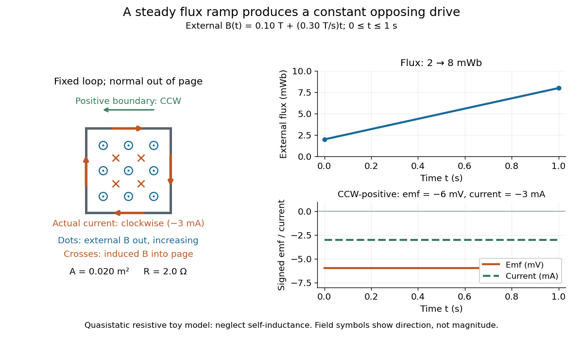
.For a computed example, a fixed single-turn loop has area and out-of-page unit normal. Prescribe an external uniform magnetic field in that direction with for . ThenIn a quasistatic resistive model with electrical resistance , neglect the loop's self-inductance and its own contribution to changing magnetic flux. Ohm's law givesThe magnetic flux rises from to while the induced electromotive force stays constant: it measures the rate of change, rather than the amount of magnetic flux. The negative sign means clockwise electric current; its magnetic field through the loop points into the page, as explained by Lenz's law. The toy model describes the interval of steady ramping, excluding switching transients at its ends.

For a moving conducting loop , the electromagnetic electromotive force instead includes the Lorentz force contribution from the local velocity of each conductor segment:This form assumes a thin-wire model with a well-defined closed contour and spanning oriented surface that move compatibly, a magnetic field satisfying Gauss's law for magnetism, and conductor speeds small compared with the speed of light. Ideal sliding contacts such as those in motional electromotive force can be treated piecewise. Arbitrary changes of electrical connections require checking the actual contour and conductor velocities; differentiating the flux through an arbitrary chosen moving path is insufficient. The velocity here describes conductor motion, not the charge carriers' drift along the wire. [ref]
https://www.feynmanlectures.caltech.edu/II_17.html#Ch17-S2. Feynman lectures, II.17.2: limits of the flux rule
.A short derivation of the fixed-loop integral statement applies Stokes theorem to the local curl equation and differentiates under the fixed surface integral. For the moving loop, the magnetic flux transport for a moving circuit adds the swept-area term to . Combining these two identities gives the moving-loop statement. This derives the integral forms from the local field law; it is not a proof of that empirical law from mathematics alone.
The useful unity is geometric: changing the magnetic field, the enclosed area, or the orientation can change magnetic flux and hence produce an electromotive force. A coil's multiple turns are accounted for by magnetic flux linkage, rather than by multiplying a single-turn flux without checking which flux each turn receives. [ref]
https://openstax.org/books/university-physics-volume-2/pages/13-1-faradays-law. OpenStax University Physics 2, §13.1: flux changes and coils
.Faraday's report read on 24 November 1831 describes opposite momentary responses when a neighboring circuit is connected and disconnected, with no continuing response while its steady electric current is maintained. These are concrete experimental roots of the changing-flux idea. The report predates the modern Maxwell equations notation used above. [ref]
Experimental Researches in Electricity, Volume 1 by Michael Faraday. Faraday, Experimental Researches in Electricity, First Series (1831), §§10–11, reprinted in volume I
.The magnetic nonrelativistic limit neglects displacement current and uses , , . Under a Galilean transformation , , its consistent field transformations are , and . Indeed and , giving covariance of the induction equation. The full charge-current transformation has ; neglecting its convective correction belongs to the magnetic quasineutral approximation, not exact relativistic electrodynamics. With , the combination is invariant. Vanishing electric field in the fluid rest frame therefore gives the ideal magnetohydrodynamic induction equation.
Use the negative curvature convention defined in curvature-sign convention in Killing derivative identities, and . Covariant derivatives of a vector obey . Hence the flat-space equivalent expressions and acquire a difference under the comma-to-semicolon prescription. Covariantizing and its Maxwell equations gives . This form respects gauge invariance. Dropping the Ricci term is generally not gauge invariant. The two expressions coincide in a Ricci-flat vacuum spacetime; vanishing matter alone with nonzero cosmological constant does not imply Ricci flatness.
Vacuum Maxwell equations without sources are invariant under , . At this is , . Electric-conductor boundary conditions are not invariant under arbitrary duality rotations; the transformed fields must be tested separately against the wall conditions.
A reductio rejects an assumption by deriving an absurd or contradictory consequence from it. In a classical mathematical proof of , assume its negation and derive a contradiction. Constructively the same argument yields the double negation of ; removing it requires an additional logical principle. This differs from proving a negation directly by deriving a contradiction from the positive assumption.
There are unlisted articles, also show them or only show them.