An optical path length measures how much propagation wave phase a path accumulates, expressed as the distance that would accumulate the same wave phase in vacuum. A centimetre in a uniform medium with refractive index has optical path length , although its geometric length remains . This makes optical path length useful whenever two contributions must arrive with matching wave phases, from an optical lens to a Michelson interferometer. [ref]
For a specified path at fixed angular frequency , the optical path length is the line integralHere is geometric arc length, and is the phase refractive index, evaluated at the same frequency everywhere. The propagation interpretation assumes a stationary linear medium with isotropy, a real positive scalar refractive index and negligible loss, on a valid geometrical optics branch. The path can curve; at sharp interfaces apply the appropriate matching conditions to each segment. A prescribed curve has a mathematical line integral, but it predicts a propagation wave phase only when it represents the physical branch. [ref] Optical fibers can require a mode wavenumber rather than the bulk refractive index along a guessed light ray. [ref]
Fix the vacuum wavelength , with frequency and vacuum wavenumber . In a locally uniform medium the wavelength is , while the frequency stays unchanged at a stationary interface. With the convention , propagation from a specified starting wave phase contributesThe relative reference includes launch wave phases and any extra wave phase from mirrors, beam splitters or coatings. Thus is a propagation contribution, not an absolute detector wave phase independent of the apparatus. If the reference contributions stay fixed, a change in optical path difference changes the phase difference by . Using the material wavelength again in this formula would count the refractive index twice. [ref]
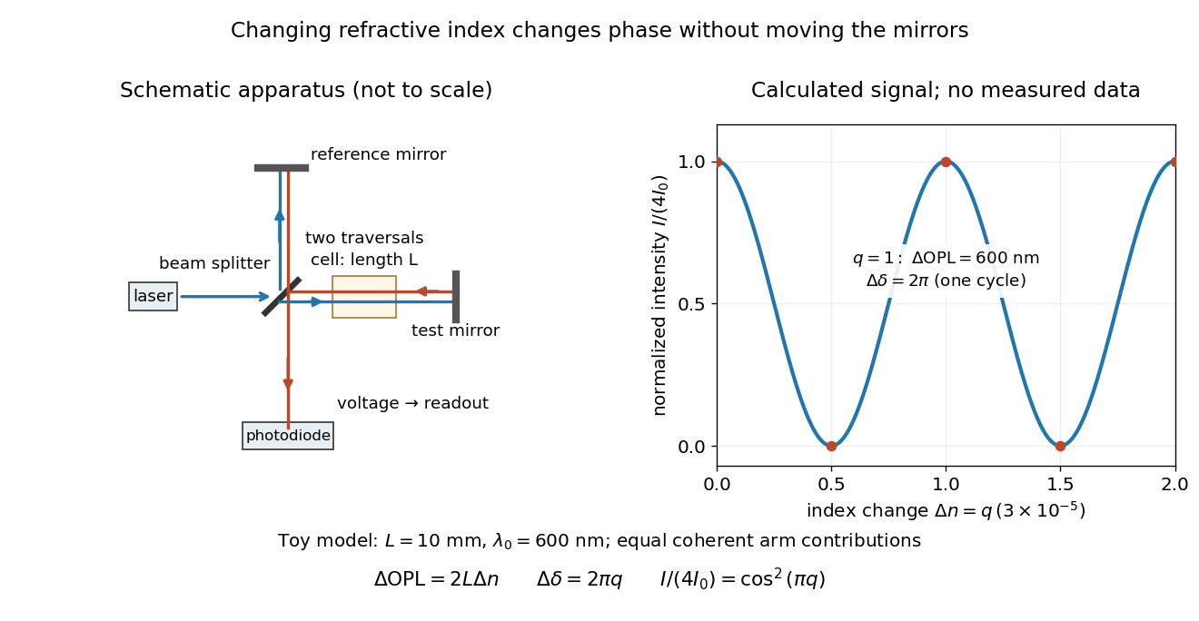
Optical path difference in a Michelson interferometer: apparatus schematic and a calculated phase difference readout
. Details. 
A motivating measurement turns invisible optical oscillations into a slowly changing electrical signal. MIT's teaching experiment uses a laser, a beam splitter, two returning mirrors, an amplified photodiode, an oscilloscope and a calibrated mirror actuator driven by a function generator. The returning beams overlap on the photodiode; one channel records detector voltage and another the actuator drive. The measured observable is the changing light intensity, including its maxima and minima, rather than direct timing of an optical cycle. A calibrated displacement per drive voltage and the spacing of the extrema relate geometric motion to the phase difference. The guide infers the laser wavelength from known actuator calibration; conversely, with independently known vacuum wavelength and ambient refractive index, the same relation calibrates mirror motion. These two unknowns cannot both be inferred from fringe spacing alone. [ref]
For a proposed change-of-medium measurement, keep the mirrors fixed and put a transparent cell of internal length in one arm. Compare its contents at refractive indices and , leaving its windows in place. At normal incidence the two traversals giveHere is the signed number of whole interference fringe cycles plus any resolved fractional cycle, counted continuously. A mirror displacement instead gives ; distinguish this double-pass factor from a single pass in a Mach-Zehnder interferometer. OpenStax's gas-cell worked example provides the same double-pass reasoning; it is a teaching calculation rather than a published measurement dataset.[ref]
An exact toy calculation makes the sensitivity visible. Stipulate , and . Then and : a full interference fringe cycle, despite unchanged geometric lengths. For a continuous change , let and choose the initial detector phase difference to be zero. Equal coherent detected arm contributions of light intensity predictThe plot is this stipulated model: gives a minimum, restores a maximum, and the reference level is chosen by adjustment of the apparatus. It contains no measured values or assigned properties of a real gas. The equivalent mirror travel in vacuum is per cycle. A single endpoint light intensity cannot distinguish from ; the continuous fringe count carries the missing information.
For an interpretable cell measurement, establish the initial phase difference with a small calibrated mirror scan, then track slow changes through successive interference fringes. Measure the dark signal and each arm separately, keep photodiode gain within its linear range, align both beams on the same region and match their linear polarizations. Monitor interferometric visibility and keep arm delays within the useful optical coherence time. Record cell length, contents, pressure and temperature; return to the starting condition to check drift. Changes in window deformation, cell length, external air or mirror position also change optical path length, so a reference cell or an independently monitored mechanical path is needed to isolate the contents' refractive index. These controls are deductions from the model, not a claim that the illustrated apparatus was operated. Loss of fringe count leaves a whole-cycle ambiguity; at an intensity extremum the first derivative with respect to phase difference vanishes, so a scan around phase quadrature is more sensitive to small changes. Broadband illumination, unstable optical coherence, vibration and strong loss can invalidate a simple one-frequency inference.
For and probability measures with finite th absolute moments,where is the ground metric and ranges over transport plans. For this is the second Wasserstein distance.
On a Polish space , probability measures with finite first moments satisfyThe supremum runs over functions with Lipschitz constant at most one. Fixing ensures integrability from the moment assumption.
In Euclidean space, push an optimal transport plan forward by . The resulting probability measures form a constant speed curve for the p-Wasserstein distance:If the plan is induced by a transport map , this becomes the displayed title formula.
On a -dimensional Hilbert space, the Von Neumann entropy is maximized uniquely by . Indeed, nonnegativity of quantum relative entropy giveswith equality exactly when .
A vector field preserves a chosen volume form when its local flow pulls back to itself. Infinitesimally this is , using the Lie derivative. The condition depends on the chosen volume form.
For thickness , radial velocity and external pressure , the leading Newtonian fluid stress tensor and incompressibility giveRadial force balance on an annular sector includes the inward projection of hoop traction and external pressure on the sloping broad faces. Together with conservation of mass it yields
A vector space over the field of complex numbers. A complex-linear map preserves addition and multiplication by complex scalars.
For complex vector spaces, an antilinear map satisfies . It is linear over the real numbers and conjugates complex scalar multiplication. This differs from two conjugate linear operators, which are related by similarity rather than conjugate-linearity.
For , put and , with . Dividing by this accumulated homogeneous growth gives and . A telescoping series then provesThis is the discrete counterpart of the integrating factor for a first-order linear differential equation.
For positive integers , some ensures that every -color finite coloring of contains a monochromatic setIt follows from the Van der Waerden theorem by mathematical induction on the number of colors. If is a bound for colors, take a long one-color arithmetic progression of length and step . Either one of has its color, giving the result immediately, or these multiples use only colors. Pull back their finite coloring to and use mathematical induction, then multiply the resulting configuration by . Enlarge the ambient finite integer interval to include all these multiples. The cases and are immediate. The parameter makes this useful for positive monochromatic solutions of a partition regular equation with arbitrary integer coefficients.
A scalar-field vacuum is a constant field at a minimum of its potential energy, with the minimum shifted to zero when discussing finite-energy classical field-theory solitons. Distinct isolated vacua allow a scalar-field kink to approach different values at the two ends of space.
Upper critical dimension of an even scalar interaction by  Codex 0 Created 2026-10-05 Updated 2026-10-07
At the Gaussian fixed point, the engineering dimension of the coupling of is . It vanishes at the upper critical dimension .
If maps the unit disc conformally to a proper simply connected domain, the nonvanishing holomorphic quotient has harmonic log modulus. Its radial mean equals . Boundary values are understood as radial limits: the standard integral-mean bound for , together with the Koebe distortion theorem lower bound , gives uniform integrability of these logarithms. Hence
The Koebe function is a univalent function from the unit disc onto . To see the image, maps the disc onto the right half-plane and . Its normalization , proves sharpness of the Koebe quarter theorem.
For a number field and a finite set of finite primes, an S-unit is an element of whose discrete valuation is zero at every prime outside . Its group is the unit group of the ring obtained by allowing denominators at . The Dirichlet unit theorem and the valuation homomorphism to show that this group is a finitely generated abelian group.
With permeability of a porous medium , the Dupuit approximation givesHere is porosity and is recharge. The low-height limit has mobility proportional to , whereas large heights have mobility proportional to . This changes both the forced filling similarity for power-law diffusion and the separable draining profile for power-law diffusion.
The Dupuit approximation treats flow in a shallow unconfined aquifer as predominantly horizontal, with hydrostatic pressure and horizontal pressure gradient independent of depth. Integrating Darcy's law over the saturated depth then gives a volume flux per unit width depending only on the groundwater height and its slope.
In Type Ia supernova cosmology, the predicted apparent magnitude depends on the common absolute magnitude and the Hubble constant only through , after choosing a fixed reference . A flat improper prior on makes the likelihood integrated over independent of , by translation of the integration variable. If the other prior factors are independent and the posterior is proper, the marginal posterior of equals its prior. An external calibration of can break this lack of identifiability.
There are unlisted articles, also show them or only show them.