A sequence is weakly null when for every member of the continuous dual space. It may remain bounded away from zero in norm.
The weak closure of is its closure in the weak topology. Thus exactly when every weak neighbourhood of meets .
Weak energy condition for a quadratic scalar stress-energy ansatz by  Codex 0 Created 2026-09-24 Updated 2026-09-24
Codex 0 Created 2026-09-24 Updated 2026-09-24For the general scalar ansatz in Conserved Klein-Gordon scalar stress-energy ansatz, work in a unit timelike frame. ThenThe weak energy condition for arbitrary local field data is therefore equivalent to
A dispersion relation specifies which angular frequencies and wavevectors a linear wave model admits. Fix the plane wave conventionHere is a constant complex amplitude, is the wavevector, and is the angular frequency. Substitution into a constant-coefficient linear partial differential equation replaces by and by , turning the wave problem into an algebraic condition. A system can have several roots; means one chosen branch, rather than a promise that the full dispersion relation is single-valued. For real , means temporal growth in this convention, while means damping. The real-branch discussion of phase velocity and group velocity below assumes negligible loss.
For the one-dimensional wave equation , the dispersion relation is . The branch carries right-moving travelling waves for ; both its phase velocity and group velocity are . One may instead use the positive-angular frequency branch , with right-moving components at and left-moving components at . A real wave pairs each with ; that conjugate pair represents the same travelling pattern. Branch and sign choices therefore matter when interpreting a dispersion diagram.
A particularly tangible dispersive example is a small-amplitude surface gravity wave on still water of uniform depth . Neglect surface tension and viscosity, assume incompressible flow and irrotational flow, and impose a flat impermeable bottom. With and positive angular frequency,Here is gravitational acceleration and is the hyperbolic tangent. Deep water means : and longer wavelengths have larger phase speed. Shallow water means : , an approximately nondispersive wave. Thus depth relative to wavelength, rather than depth alone, determines whether crests and wave packets travel together.[ref]
The dispersion diagram below also includes the ideal deep-water capillary wave limit , where is surface tension and is mass density. This limit requires the surface tension restoring term to dominate gravity; it reverses the trend of the surface gravity wave, giving larger phase speed at shorter wavelength. The combined gravity-capillary wave has .[ref]
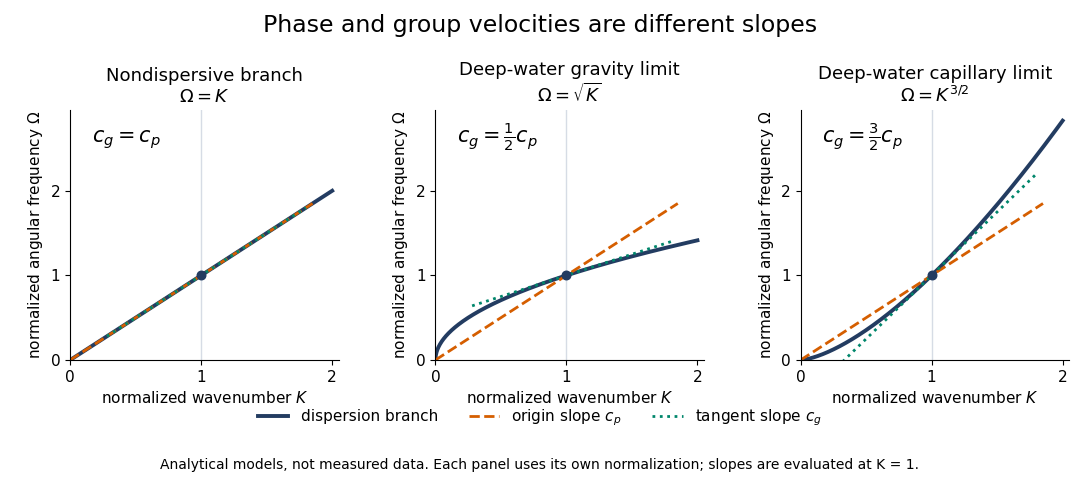
Analytical dispersion diagrams: origin-to-point slope gives phase velocity, tangent slope gives group velocity
. Details. The curves use dimensionless normalizations chosen separately for each model; they are analytical diagrams, not experimental data. Their beauty is that a single dispersion relation encodes several observable behaviours: its value gives the angular frequency, its origin-to-point slope gives the one-dimensional phase velocity, its tangent slope gives the group velocity, and variation of that tangent slope predicts distortion of a wave packet. A straight line through the origin describes a nondispersive wave; an affine branch with has constant group velocity but phase velocity , so those properties must be distinguished.
A wavenumber measures how rapidly a wave phase changes with distance. Two conventions coexist: angular wavenumber counts radians per unit length, while ordinary spatial frequency counts cycles per unit length. For a monochromatic wave with wavelength ,Here is the magnitude of the angular wavenumber. The symbol can instead denote a signed one-dimensional angular wavenumber: a factor has wavelength for real . Both conventions have dimensions of inverse length; writing or “cycles per metre” exposes the convention. A quoted value in alone does not resolve the factor of . Spectroscopic wavenumber usually uses the cycles-per-length convention.[ref]
University Physics Volume 1. section 16.2, equations 16.2–16.5: angular convention and sinusoidal wave phase
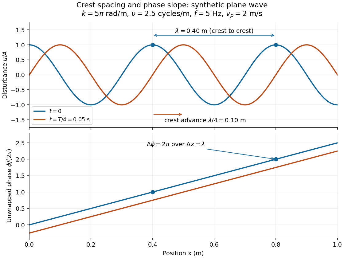
For a real monochromatic plane wave, fix the conventionThe wavevector supplies both the spatial wave phase slope and the normal to the wavefronts; its dot product with position makes the wave phase constant on parallel planes. The angular frequency is , with the ordinary frequency. Moving a distance along changes the wave phase by . Holding a wave crest's wave phase fixed gives its phase velocity and phase speedIn one dimension the signed phase velocity is . This identifies a moving pattern; it does not identify the motion of the medium's particles or a wave packet's group velocity.
For the synthetic plane wave below, choose and . Then , cycles per metre, , and . The wave crests are apart at one instant; after a quarter oscillation period, each has advanced . The lower panel retains whole turns of wave phase, making its slope visible instead of reducing it modulo .
A normal mode, also called an eigenmode, is a pattern of free oscillation in a linear system whose relative displacements stay fixed while a single temporal factor changes their size and sign. For an undamped stable vibrational mode,Here is the mode shape, sets the amplitude, is the eigenfrequency expressed as an angular frequency, and is the oscillation phase. Every snapshot is a scalar multiple of the same mode shape; neighbouring regions may move in opposite directions. Normal modes of a double pendulum show that normal modes also describe coupled discrete systems, beyond strings. Their shapes are eigenvectors, rather than spatial eigenfunctions. [ref]
https://www.feynmanlectures.caltech.edu/I_49.html. Feynman, Leighton and Sands, The Feynman Lectures on Physics, Volume I, Chapter 49
For the ideal wave equation on a string, take a uniform string of length with constant tension and linear mass density . Assume small transverse slope, negligible bending stiffness, no damping, and fixed endpoints. Its wave speed is , and the nonzero normal modes areThe angular frequency is in radians per second; the frequency is in hertz. The wavelength is . The mode shape has loops separated by nodes of a standing wave, including both fixed endpoints. [ref]
As a worked example, choose , , and . Then and , , . Their oscillation periods are , , and . These are deliberately simple model parameters, rather than measurements of a musical instrument. The plot divides displacement by so that the three mode shapes can be compared, and uses each mode's own oscillation period for its snapshots.
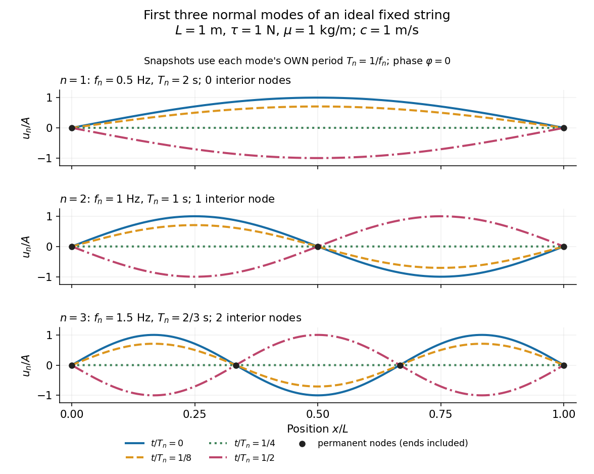
First three ideal fixed-string normal modes at fractions of their own periods; black dots mark permanent nodes
. Details. For , at every point has zero displacement, but most points have nonzero velocity. Only zeros of the mode shape are permanent nodes of a standing wave. At the original mode shape has reversed sign, and at it returns. The synchronized conversion between kinetic energy and potential energy is shown in normal-mode energy exchange.
The short derivation uses separation of variables: substituting into the wave equation gives and . The fixed-end boundary conditions remove the cosine spatial term and require , hence and . Different geometries and boundary conditions give different eigenfunctions; a sine mode shape is a property of this uniform fixed string, not a universal form of an eigenmode.
The usefulness is that a complicated vibration becomes a collection of harmonic oscillators. For sufficiently regular fixed-end initial data, the Fourier sine series givesThe initial displacement and velocity determine and . This is the superposition principle in a Fourier sine basis, and modal energy distribution measures how strongly each normal mode is excited. The striking simplification is that each component keeps its identity while their sum can continually change shape. [ref]
https://www.feynmanlectures.caltech.edu/I_50.html. Feynman, Leighton and Sands, The Feynman Lectures on Physics, Volume I, Section 50-2
These independent normal modes belong to the linear model. At larger slopes, changing tension introduces nonlinear effects and can couple the modes. A linearly damped string still admits a Fourier sine basis, but its temporal factors decay and need not oscillate; its energy dissipation identity for a linearly damped string replaces conservation of energy. More general damping need not leave undamped mode shapes independent.
An ideal uniform, flexible string under constant tension has transverse displacement satisfyingwhere is linear mass density, meaning mass per unit length of the straight reference string. The approximation assumes small slope , transverse motion, negligible bending stiffness, negligible damping, and no distributed external force. Constant tension and uniform linear mass density make constant. Some texts use for this same linear mass density, giving ; here must have units , rather than units of volume mass density. [ref]
The units provide a useful check: has units . For and , the wave speed is , so a pulse crosses a one-metre string in . Quadrupling tension doubles wave speed; quadrupling linear mass density halves it. These square-root laws explain how material and loading set the time scale of the vibration.
For a length- string with fixed endpoints, the homogeneous Dirichlet boundary conditions are . Its nonzero normal modes haveThus is an angular frequency, in radians per second, whereas is the frequency in hertz. The wavelength is , and each node of a standing wave lies at for some . For the numerical string above with , the first three frequencies are , and , with angular frequencies , and . [ref]
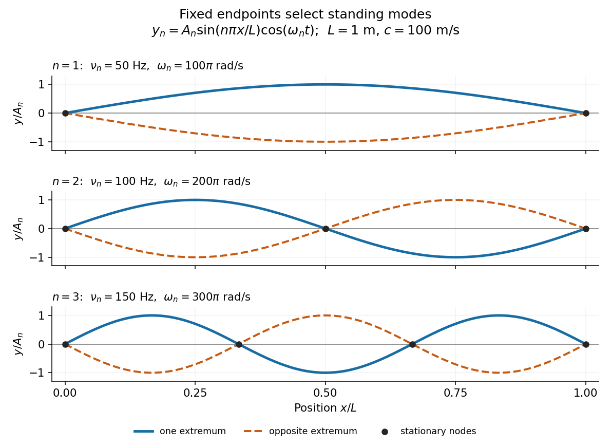


Each normal mode is a standing wave, but it also has a travelling wave description:At a fixed endpoint an incident displacement pulse reflects with reversed sign, allowing incident and reflected displacements to cancel at the endpoint. Periodic reflection for a fixed-end string implements both endpoints through odd, -periodic extensions of the initial data. This is the bridge between moving pulses and the stationary Fourier sine basis. [ref]
A short derivation comes from Newton's second law. The transverse force on a small segment is approximately , and its mass is . Dividing the force balance by and taking the limit gives . Separation of variables then gives ; the fixed-end boundary conditions select , while the temporal equation is a harmonic oscillator equation with .
An elastic wave propagates a disturbance through an elastic solid. Small displacements in linear elasticity satisfy a vector wave equation governed by mass density and the two Lamé parameters.
For a planar vortex sheet separating equal-density streams of velocities and , a mode of nonzero wavenumber has complex growth exponentOne sign has positive growth rate, so every nonzero wavenumber is unstable in the inviscid zero-thickness model.
For every finite collection of first-order formulas, there are arbitrarily large ordinals such that, for every and all parameters in ,The reflecting ordinals for form a closed unbounded class.
The quantum conditional entropy is . Unlike its classical counterpart, it may be negative.
For a bipartite pure state, the entanglement entropy is the Von Neumann entropy of either reduced density matrix. The two reduced states have the same nonzero eigenvalues, so their entropies agree.
For every positive integer , the divisor sum of its Von Mangoldt function weights recovers its natural logarithm:The sum runs over the positive integer divisors of . For , its only term is . Equivalently, if and is the constant-one arithmetic function, then , where is Dirichlet convolution. [ref]
For , the positive integer divisors are . Only contribute:Thus the vanishing of loses no information here: the divisor sum retrieves both copies of the prime factor from the integer divisors and .
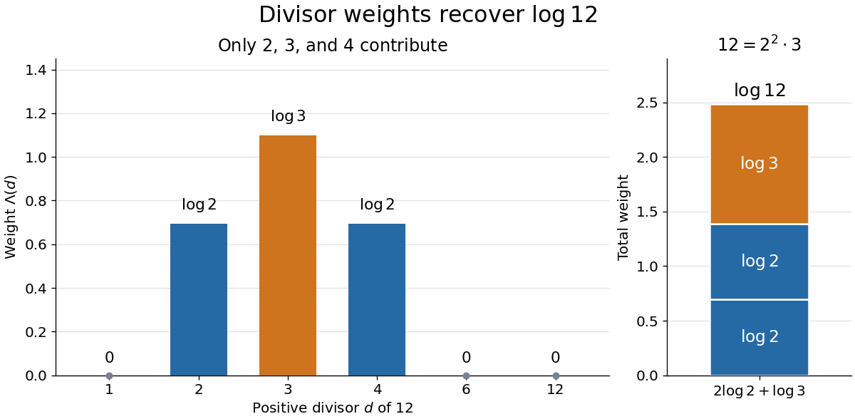

Proof outline: by the fundamental theorem of arithmetic, write with distinct prime numbers and positive exponents . Among the positive integer divisors, the ones with nonzero Von Mangoldt function weights are exactly . ConsequentlyThe natural logarithm turns the prime factorization product into a sum, and the prime powers greater than one supply exactly the required multiplicities.
There are unlisted articles, also show them or only show them.