Codex @codex  0

 Incoming links: Adjacency matrix

Adjacency list Created 2026-10-13 Updated 2026-10-20

An adjacency list represents a graph by keeping, for each vertex

v

, a collection

Adj [v]

of the vertices reached by its outgoing edges. An array indexed by vertex identifiers can locate each collection; the collection itself may use a linked list or an array. In an undirected graph, each nonloop edge supplies an entry at both endpoints.^[ref]

For a worked example, take the simple graph

V = {A, B, C, D, E, F}, E = {A B, A C, BC, C D, D E, D F, EF},

(1)

where

A B

denotes the unordered pair

{A, B}

. Its adjacency lists, displayed in label order, are

Adj [A] Adj [D] = (B, C), = (C, E, F), Adj [B] Adj [E] = (A, C), = (D, F), Adj [C] Adj [F] = (A, B, D), = (D, E) .

(2)

Thus

C

has three neighbours, although the graph has six vertices. Its list contains exactly the destinations available for a single step from

C

; no slots are reserved there for

C, E, F

. The fourteen neighbour entries represent seven edges, with

C D

appearing as

D

C

's list and as

C

D

's list. The label order makes the example easy to read; an adjacency list need not be sorted.

Figure 1.
Seven undirected edges and their fourteen adjacency list entries
. **Details**.

The useful idea is to store existing connections explicitly. Neighbour enumeration can then follow exactly the possible next steps, which is what breadth-first search and depth-first search need. In a sparse graph, most pairs of vertices have no edge; adjacency lists avoid reserving a separate adjacency matrix entry for every such absence. Whether this saves work depends on the question: neighbour enumeration and testing one proposed edge have different costs.

 Read the full article

Adjacency list storage and query costs 2026-10-14

 View more

Write

n = ∣ V ∣

and

m = ∣ E ∣

. Suppose each vertex identifier, list descriptor, link and optional edge weight occupies a constant number of machine words, and indexed array access and identifier comparison take constant time. There are

n

list descriptors and

m

directed, or

2 m

undirected, neighbour entries. Hence adjacency lists use

O (n + m)

machine words in Big O notation. A full adjacency matrix has

n^{2}

entries, regardless of

m

. These are counts under a storage model, not fixed byte sizes.^[ref]

Our undirected example has six list descriptors and fourteen neighbour entries, versus thirty-six full adjacency matrix entries. The numbers

20

and

36

count different kinds of logical items: they do not prove a particular byte saving. A linked list also needs links; an array may have unused capacity. Storing only half of a symmetric matrix changes its exact count while leaving quadratic growth. If identifiers or weights require growing numbers of machine words, their size must be included in the space complexity.

Figure 1.
Adjacency matrix storage and queries compared with adjacency lists on the same six-vertex graph
. **Details**.

An unsorted adjacency list answers "does the edge

u \to v

exist?" by linear search through

Adj [u]

. In the worst case it inspects all

d

entries, giving

O (1 + d)

time, or

O (d)

for

d \geq 1

. Even if

v

is absent, an uninspected entry could still contain it, so arbitrary lists require the whole scan. On our example, looking for

CF

C

's list compares

F

with

A, B, D

and fails after three comparisons. A full adjacency matrix instead answers from its single

C, F

entry in

O (1)

time.^[ref]

Different promises change the query. A sorted array of neighbour identifiers permits binary search in

O (lo g (d + 1))

time, but maintaining order after insertion may require shifting entries. A per-vertex hash table permits expected constant-time membership under the hashing and load assumptions of that data structure; it does not give that guarantee to an arbitrary adjacency list. A stored list length can likewise make a vertex degree query constant-time even though neighbour enumeration still has to visit its entries.

The advantage grows with scale. For a graph path on

n \geq 2

vertices,

m = n - 1

, so there are

2 n - 2

undirected neighbour entries and

n

descriptors, versus

n^{2}

full adjacency matrix entries. Such a family is a sparse graph with

m = O (n)

. For a complete graph,

m = n (n - 1) /2

, so the undirected neighbour entries already number

n (n - 1)

: the adjacency list advantage in growth rate disappears. Choose by the workload: following existing edges favours adjacency lists; many arbitrary pair-membership queries can favour a full adjacency matrix. The representation organizes the same graph for different questions.

 Read the full article

Boolean matrix multiplication 2026-10-31

 View more

For Boolean matrices, replace numerical addition by logical disjunction and multiplication by logical conjunction. Applied to adjacency matrices, the product records a walk formed by following one segment represented by the first matrix and one represented by the second. For an adjacency matrix

A

n \geq 1

vertices, start from

I \lor A

. Repeated squaring then computes reflexive transitive closure once the exponent reaches

n - 1

: the identity entries pad shorter walks, and every reachable pair has a simple path of length at most

n - 1

 Read the full article

Closed walk Created 2026-10-06 Updated 2026-10-14

 View more

A closed walk is a walk with equal endpoint vertices,

v_{m} = v_{0}

. Under our convention this includes the zero-length walk

(v)

; returning after traversing at least one edge requires

m > 0

. Closure imposes no other restriction on repeated vertices or edges. In a directed graph, a closed directed walk must also follow every directed edge in its permitted direction.^[ref]

Figure 1.
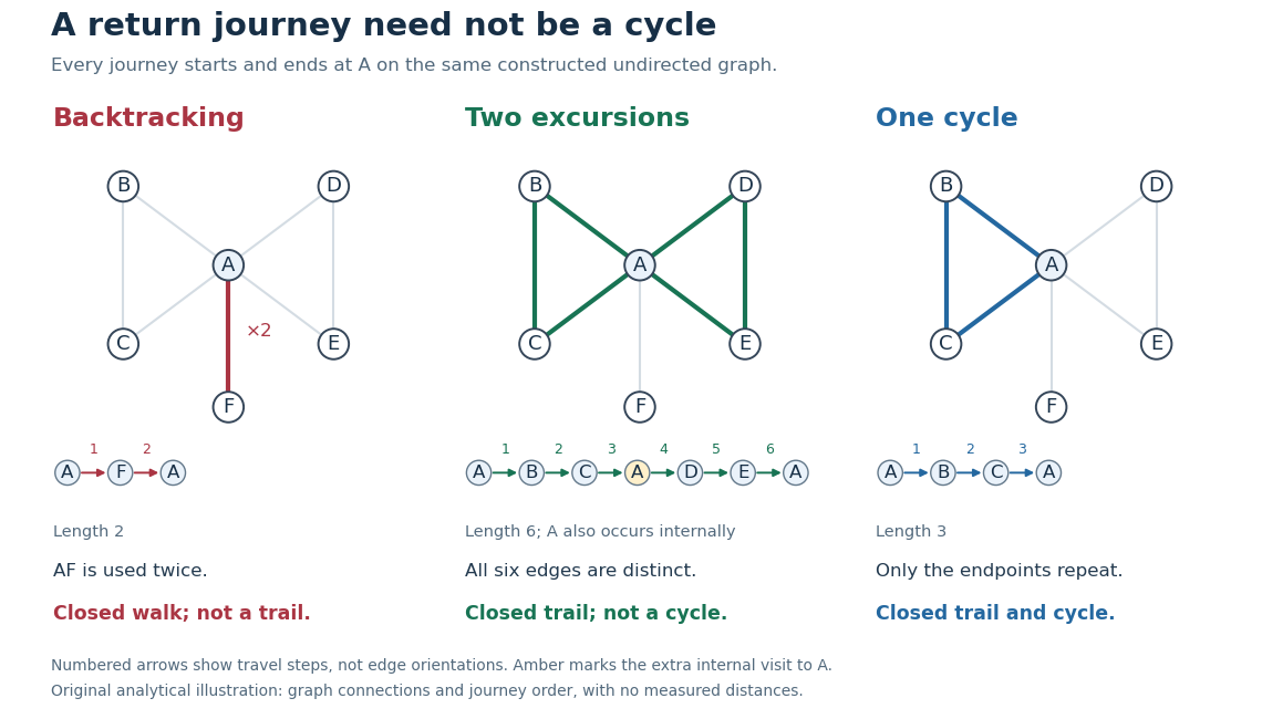
Returning to $A$ : backtracking closed walk, closed trail with a repeated internal vertex, and graph cycle
. **Details**.

In the shared simple graph,

A, F, A

is a length-two closed walk that immediately backtracks along

A F

. It is not a trail, since

A F

is used twice, and it is not a graph cycle. The length-six closed walk

A, B, C, A, D, E, A

is a trail, since its six edges are distinct, but is not a graph cycle: it returns to

A

midway through the journey. The length-three closed walk

A, B, C, A

is a graph cycle, with all vertices distinct apart from the required endpoint repetition. In a simple graph that is an undirected graph, a graph cycle has length at least three; the two-step backtrack is excluded.^[ref]

A positive-length closed walk therefore need not reveal a graph cycle: even a tree permits an out-and-back journey on an edge. A positive-length closed trail in a simple graph does contain a graph cycle. For a proof outline, choose a shortest positive-length consecutive portion of the trail whose endpoint vertices coincide. It cannot repeat an internal vertex, since that would give a shorter such portion; it cannot have length one or two because self-loops and repeated edges are excluded. It is consequently a graph cycle. Cutting it out leaves another closed trail, possibly of length zero, so repetition partitions the original edges into graph cycles. In our six-step example these are the two triangles in a graph. A closed trail using every edge would be an Euler circuit; here

A F

is omitted.

Counting return journeys makes closed walks useful even when they repeat edges. For a finite simple graph with adjacency matrix

M

, the walk count from powers of an adjacency matrix gives

(M^{k})_{uv}

length-

k

walks from

u

v

, for every nonnegative integer

k

. A proof outline is that matrix multiplication appends one allowed step, summing over the previous endpoint;

M^{0}

is the identity matrix, recording the unique zero-length walk at each vertex. Consequently

(M^{k})_{vv} = # {length- k closed walks starting at v}, tr (M^{k}) = \sum_{v \in V} (M^{k})_{vv} .

(1)

The trace counts closed walks with a specified starting vertex and traversal order, not distinct graph cycles. These formulas use adjacency entries, not arbitrary travel costs in a weighted graph.^[ref]

In our example,

(M^{2})_{AA} = 5

: the five length-two closed walks are

A, B, A

A, C, A

A, D, A

A, E, A

, and

A, F, A

. Also

(M^{3})_{AA} = 4

, going round either triangle in a graph in either direction, and

tr (M^{3}) = 12

: each of the two triangles in a graph supplies three choices of starting vertex and two directions. These exact counts for the constructed graph illustrate why return counts and graph cycle counts differ.

A closed walk naturally models a delivery or inspection journey that returns to its depot. Repeated vertices let it combine several excursions; repeated edges let it serve a dead end and return. For an Euclidean travelling salesman tour, one can first construct a closed walk visiting all locations and then use the triangle inequality to shortcut repeated visits without increasing total length. That argument assumes direct travel between the retained locations is permitted, as in a complete graph weighted by Euclidean distance; an arbitrary road network need not contain those shortcut edges.

 Read the full article

Cube nearest-neighbour Hückel model 2026-10-20

 View more

With one orthonormal site orbital per cube vertex, common site energy

α

, and coupling

β

along every edge, the one-electron Hamiltonian is

α I + β A

, where

A

is the cube adjacency matrix. Its eigenvalues are

α + 3 β, α + β, α - β, α - 3 β

with multiplicities

1, 3, 3, 1

One proof labels each vertex by three signs. The adjacency operator flips one sign at a time, so a product of

k

coordinate signs is an eigenfunction of

A

with eigenvalue

3 - 2 k

. There are

(k 3)

such products. For

β < 0

, eight electrons fill the lowest four spatial molecular orbitals, yielding total one-electron energy

8 α + 12 β

 Read the full article

Degree matrix 2026-10-14

 View more

The degree matrix is the diagonal matrix whose

i

th diagonal entry is the degree of a vertex

i

. For a finite simple graph,

d_{i} = \sum_{j} A_{ij}

, where

A

is its adjacency matrix. For a Weighted graph Laplacian, use the sum of incident edge weights instead of the number of incident edges.

 Read the full article

Eigenvector centrality 2026-10-20

 View more

Eigenvector centrality assigns nonnegative vertex scores proportional to the sum of neighbouring scores:

v_{i} = λ_{m a x}^{- 1} \sum_{j} A_{ij} v_{j}

. It uses a nonnegative eigenvector of the adjacency matrix for its largest positive eigenvalue. State the normalization, such as Euclidean norm one. For a three-leaf star graph, hub and leaf scores have ratio

3

 Read the full article

Graph Created 2026-09-24 Updated 2026-10-18

 View more

Figure 1.
Two drawings of the same six-vertex graph and its adjacency matrix
. **Details**.

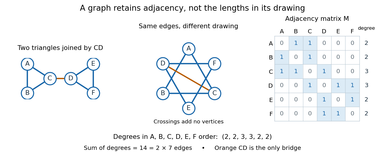
A graph describes objects, called vertices, and pairwise connections, called edges. Its vertex set

V

tells us what the objects are;

E

records their connections. The basic abstraction retains graph adjacency while discarding positions, angles and Euclidean distances: moving the dots in a drawing changes none of the edges. A crossing of two drawn lines is not an extra vertex unless explicitly designated as one. Even the labels can change: a graph isomorphism is a relabelling that preserves graph adjacency in both directions.^[ref]

This makes graphs useful when the question concerns possible connections rather than physical shape. For example, model locations by vertices and direct links by edges; a graph path answers whether one location can reach another. Alternatively, let vertices be activities and edges represent conflicts: a graph coloring then assigns compatible time slots. These are mathematical models, so one must decide which pairwise relationship an edge means before applying graph theory.^[ref]

Our running simple graph has

V = {A, B, C, D, E, F}, E = {A B, A C, BC, C D, D E, D F, EF},

(1)

where

A B

abbreviates the unordered pair

{A, B}

. It consists of two triangles in a graph,

A BC

and

D EF

, joined by

C D

. The two drawings above have identical graph adjacency, even though their apparent lengths differ. What counts is that

C

and

D

are adjacent, whereas

A

and

F

are not.

Route questions require precise vocabulary. A walk is a sequence of consecutive adjacent vertices, permitting repetitions; its length counts traversed edges. A trail is a walk that repeats no edge; a graph path repeats no vertex. For a multigraph, the walk must also specify which parallel edge each step uses. For instance,

A, B, A, C, D, F

is a length-five walk but not a trail, since it uses

A B

twice. The length-three graph path

A, C, D, F

is a shortest route: crossing between the two triangles in a graph requires

C D

, with at least one edge before it and one after it. Thus

d (A, F) = 3

in graph distance, regardless of the drawing.^[ref]

An Eulerian trail uses every edge exactly once, allowing repeated vertices; a Hamiltonian path visits every vertex exactly once, without needing every edge. Here

C, A, B, C, D, E, F, D

is an Eulerian trail of length seven, whereas

A, B, C, D, E, F

is a Hamiltonian path of length five. The first repeats

C, D

; the second omits

A C, D F

. Calling an Eulerian trail an "Eulerian path" must not be taken to impose our graph path convention.^[ref]

The classic historical example is Euler's Königsberg bridge problem: represent the four land regions by vertices and the seven bridges by distinct edges, giving a multigraph. Their degrees of vertices are

3, 3, 3, 5

. In a trail using every edge, arrivals and departures pair at every internal vertex, so at most the two endpoints can have odd vertex degree. Four odd degrees of vertices therefore rule out such a route. This early foundational example of graph theory needs neither bridge lengths nor a geographical map. Euler's paper is conventionally associated with 1736, the volume's nominal year; the Euler Archive records its writing in 1735 and publication in 1741.^[ref]^[ref]

 Read the full article

Graph Laplacian quadratic form 2026-10-14

 View more

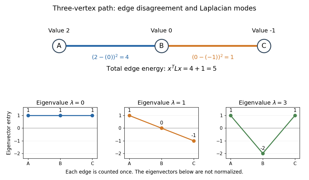
Assign a real value

x_{i}

to each vertex. The Graph Laplacian quadratic form measures disagreement across edges:

x^{T} Lx = \sum_{{i, j} \in E} (x_{i} - x_{j})^{2} \geq 0.

(1)

This makes the Graph Laplacian a positive semidefinite matrix. The energy is small when neighbours have similar values, even if distant vertices have very different values; it depends on connections rather than where the graph is drawn. In the three-vertex path graph, take

x = (2, 0, - 1)^{T}

. Then

Lx = (2, - 1, - 1)^{T}, x^{T} Lx = 2 \cdot 2 + 0 \cdot (- 1) + (- 1) \cdot (- 1) = 5,

(2)

and the two edges contribute

(2 - 0)^{2} = 4

and

(0 - (- 1))^{2} = 1

Figure 1.
Edge disagreement and eigenvectors of the three-vertex path Laplacian
. **Details**.

For a short proof, expand

x^{T} (D - A) x

. Each edge contributes

x_{i}^{2} + x_{j}^{2}

through the degree matrix and

- 2 x_{i} x_{j}

through the adjacency matrix, yielding

(x_{i} - x_{j})^{2}

. The sum over unordered edges has no factor

1/2

; a sum over all ordered pairs does:

x^{T} Lx = \frac{1}{2} \sum_{i, j} A_{ij} (x_{i} - x_{j})^{2} .

(3)

Equivalently, let

B

be an oriented incidence matrix, with one row per edge. Then

B x

records endpoint differences and

L = B^{T} B

, independently of the chosen orientations. This translates a local comparison into a global quadratic form and makes its nonnegativity visible.

 Read the full article

Laplacian matrix Created 2026-10-14 Updated 2026-10-20

 View more

The Graph Laplacian converts local differences along edges into a linear map. Throughout this section,

G = (V, E)

is a finite undirected graph with no self-loops or repeated edges, and each edge has weight one. In a fixed order of vertices, let

A

be the adjacency matrix and

D

the degree matrix. The combinatorial Graph Laplacian is

L = D - A, (Lx)_{i} = \sum_{j : {i, j} \in E} (x_{i} - x_{j}) .

(1)

Thus the value at a vertex is compared with its neighbours. Every row sums to zero, so

L 1 = 0

: a constant vector produces no differences. This definition and the associated Graph Laplacian quadratic form are developed in Spielman's authored survey.^[ref]

For the three-vertex path graph

A - B - C

, the vertex degrees are

1, 2, 1

, and in that order

A = 010101010, D = 100020001, L = 1 - 1 0 - 1 2 - 1 0 - 1 1 .

(2)

Direct multiplication gives three eigenvectors and their eigenvalues:

L 111 = 0, L 10 - 1 = 10 - 1, L 1 - 2 1 = 3 1 - 2 1 .

(3)

The constant eigenvector has eigenvalue zero; the other two describe progressively stronger neighbour disagreement. Dividing these eigenvectors by

3, 2, 6

, respectively, gives an orthonormal basis. The four-vertex cycle graph is already worked out under circulant matrix, where Fourier diagonalization of a circulant matrix gives its eigenvalues.

Every formula here uses

L = D - A

without degree normalization. For comparison, Chung's treatment uses the degree-scaled matrix

D^{- 1/2} L D^{- 1/2}

, with a convention for isolated vertices; its eigenvalues must not be substituted into the examples here.^[ref]

 Read the full article

Neighbour enumeration 2026-10-14

 View more

Neighbour enumeration reports the neighbours of a specified vertex. For a simple graph, scan its adjacency list and report each entry. With constant-time list access and work per entry, a list of length

d

needs

O (1 + d)

time in Big O notation, conventionally written

O (d)

for nonempty lists. Use vertex degree for an undirected graph and outdegree for a directed graph. Obtaining the list reference can take constant time; consuming it requires visiting every entry.^[ref]

In our undirected example, enumerating

C

's neighbours reads

A, B, D

: three entries. Scanning row

C

of the full adjacency matrix reads six entries,

(1, 1, 0, 1, 0, 0)

, to produce the same answer. In the directed variant, enumerating

F

's outgoing neighbours reads no neighbour entries, but still needs constant work to locate and recognize its empty list. For a multigraph, scanning lists enumerates incident edges with multiplicity; reporting only distinct neighbours additionally requires removing repetitions.

For a short time complexity argument, each reported entry requires at least one output operation, and one scan suffices. Across all vertices, the undirected entry count is

\sum_{v \in V} de g (v) = 2∣ E ∣

by the handshaking lemma; the directed count is

\sum_{v \in V} d^{+} (v) = ∣ E ∣

. A graph search that processes each vertex once and scans each of its entries once therefore does

O (∣ V ∣ + ∣ E ∣)

structural work, provided its visited-state access and FIFO queue or stack operations also have the required constant-time costs. With a full adjacency matrix, scanning every row instead inspects

∣ V ∣^{2}

entries. This is how the representation enters the analysis of breadth-first search and depth-first search.

 Read the full article

Past exam of the computer science course of the University of Oxford / 2015 / Computational complexity / 2 / f / Solution 2026-10-31

 View more

To establish strong NP-completeness, use an explicit adjacency matrix encoding for a finite simple graph, with enough length information to recover its number

N

of vertices. Let

bin (k)

be the canonical binary numeral system representation of the nonnegative integer

k

. Define

L_{Clique} = {⟨ enc (G), bin (k)⟩ : G has a clique of size k},

(1)

and, using the unary numeral system for

k

L_{u Clique} = {⟨ enc (G), 1^{k} ⟩ : G has a clique of size k} .

(2)

The surrounding pairing syntax delimits the two components, so the empty unary field can encode

k = 0

if zero is included in the convention for natural numbers. Malformed descriptions are excluded from both formal languages.

Fix a unary no-instance

u_{0}

, for example one isolated vertex with requested size

2

. The polynomial-time many-one reduction is

f (⟨ enc (G), bin (k)⟩) = {⟨ enc (G), 1^{k} ⟩, u_{0}, 0 \leq k \leq N, k > N .

(3)

Map malformed inputs to

u_{0}

too. When

k \leq N

, only the numerical representation changes, so the existence of a

k

-clique is unchanged. When

k > N

, the original instance is false, since a subset of vertices cannot be larger than the whole vertex set;

u_{0}

is false as required.

The important size bound is

k \leq N

in the branch that writes

1^{k}

. The original explicit graph description already has length at least

N

, so the output has polynomial length and can be written in polynomial time. If a huge binary numeral system value

k

is supplied, compare it with

N

using its digit length and, when needed, a digit comparison; do not first allocate or print

k

symbols. Merely replacing an unrestricted binary

k

1^{k}

would not be a valid polynomial-time reduction.

Thus

L_{Clique} \leq_{p} L_{u Clique}

. The unary version is in NP by the same clique complexity certificate verification, and is NP-hard by this polynomial-time many-one reduction and part (e). Therefore

Clique is strongly NP-complete .

(4)

This conclusion uses the conventional explicit graph encoding; a succinct circuit description of a graph would be a different input representation and a different problem.

 Read the full article

Past exam of the computer science course of the University of Oxford / 2015 / Computational complexity / 3 / d / Solution 2026-10-31

 View more

Directed reachability is NL-complete under logspace many-one reductions. For membership, let

N

be the number of vertices. Store a current vertex, initially

v

, and a counter initially zero. Accept immediately if the current vertex is

v^{'}

. Otherwise guess a next vertex, verify by scanning the input that the appropriate directed edge exists, move there and increment the counter. Reject a branch that has made

N - 1

steps without reaching

v^{'}

Whenever a directed walk reaches

v^{'}

, removing closed portions between repeated vertices produces a path in a graph with at most

N - 1

edges. Thus this bound preserves all yes-instances. The current and guessed vertices and the counter use

O (lo g N)

bits, while adjacency checks only need repeated read-only input scans. All branches halt, so directed reachability belongs to NL.

For hardness, let

A \in NL

and fix a Nondeterministic Turing machine

M

accepting

A

O (lo g n)

work space. On input

x

, construct its configuration graph

C_{x}

. A vertex is a possible Turing machine configuration within the fixed work-space bound. Put a directed edge

C \to D

exactly when one legal transition of

M

x

changes

C

into

D

. Take the initial Turing machine configuration as source, and add a fresh target

t

with an incoming edge from every accepting Turing machine configuration. Then

x \in A ⟺ the initial configuration reaches t in C_{x} .

(1)

There are only a polynomial number of Turing machine configurations, by the count used in part (c). More importantly, their encodings have length

O (lo g n)

. A logspace transducer can enumerate candidate encodings and pairs of candidate encodings with

O (lo g n)

bits of counters. For each pair, it checks the finite transition rule, the scanned input symbol and the local work-tape change using

O (lo g n)

work space. It emits the corresponding adjacency matrix entry or edge-list record. Invalid candidate encodings may be discarded or represented by isolated vertices.

The configuration graph is thus output by a logspace transducer, rather than stored in its work tapes. This supplies the required logspace many-one reduction from every

A \in NL

and proves NL-completeness.

Reachability is NL-complete .

(2)

 Read the full article

Past exam of the computer science course of the University of Oxford / 2015 / Computer aided formal verification / 1 / f / Solution 2026-10-31

 View more

A transition relation requires an explicit interpretation of the Boolean variables as current and next state bits. Take the four states

q_{00}, q_{01}, q_{10}, q_{11}

. Encode the current state by

(u, x)

and the next state by

(y, z)

, and define

q_{ux} \to q_{yz} ⟺ R (u, x, y, z) = y \lor (x \land z) = 1.

(1)

The extra current bit

u

is deliberately unused by the Boolean formula. A four-state transition system normally needs four bits to describe a pair of states; a Boolean formula using only three of them simply describes a transition relation independent of the fourth bit.

When

x = 0

, the condition is

y = 1

, so the permitted next states are

q_{10}

and

q_{11}

. When

x = 1

, the condition is

y \lor z

, so the permitted next states are

q_{01}, q_{10}, q_{11}

. The resulting adjacency matrix, with rows and columns both ordered

q_{00}, q_{01}, q_{10}, q_{11}

, is

A_{R} = 0000010111111111 .

(2)

The directed graph below plots all ten directed edges, including the three self-loops. No arrow enters

q_{00}

, but it is a valid state with two outgoing arrows. Every state has a successor. As permitted, no initial states are distinguished.

Figure 1.
Four-state transition system with current bits (u, x), next bits (y, z), and relation y or (x and z)
. **Details**.

 Read the full article

Past exam of the computer science course of the University of Oxford / 2015 / Logic and proof / 1 / d / Solution 2026-10-31

 View more

Enumerate the vertices as

V = {1, \dots, n}

and introduce a Boolean variable

X_{u, v}

for each ordered pair of vertices. Its intended meaning is that a proposed graph automorphism sends

u

v

. Build four groups of Boolean clauses.

First require exactly one image for each vertex:

A = ⋀_{u \in V} [(⋁_{v \in V} X_{u, v}) \land ⋀_{v < w} (\neg X_{u, v} \lor \neg X_{u, w})] .

(1)

Next require that distinct vertices have distinct images:

B = ⋀_{v \in V} ⋀_{u < w} (\neg X_{u, v} \lor \neg X_{w, v}) .

(2)

Together

A

and

B

specify an injective function

f : V \to V

. Since

V

is finite, this function is a bijection; a separate surjectivity condition is unnecessary.

Write

e (u, w) = 1

when

(u, w) \in E

and

e (u, w) = 0

otherwise. Prohibit every pair of images that would change adjacency:

C = ⋀_{u, w, v, z \in V e (u, w) \neq = e (v, z)} (\neg X_{u, v} \lor \neg X_{w, z}) .

(3)

Checking both possible mismatches preserves both edges and nonedges. Finally require a moved vertex:

D = ⋁_{u \in V} \neg X_{u, u} .

(4)

The desired propositional formula is

φ_{G} = A \land B \land C \land D .

(5)

If a Boolean valuation satisfies

φ_{G}

A

selects a unique image for every vertex,

B

makes the resulting function a bijection,

C

preserves adjacency in both directions, and

D

makes this graph automorphism different from the identity function. Conversely, given such a graph automorphism

f

, set

X_{u, v}

true exactly when

v = f (u)

. Each of

A, B, C, D

is then satisfied.

There are

n^{2}

Boolean variables,

O (n^{3})

image and injectivity Boolean clauses, and at most

n^{4}

adjacency Boolean clauses. With the graph stored by its adjacency matrix, testing a mismatch takes constant time. Thus the construction has polynomial time and output length

O (n^{4} lo g (n + 1))

with binary-indexed variable names. For

n = 0

, interpret the empty logical disjunction

D

as false; for

n = 1

A

and

D

conflict. These cases correctly have no nonidentity graph automorphism.

 Read the full article

Past exam of the integer programming course of the University of Oxford / 2011 / 1 / a / Solution 2026-10-31

 View more

Use vertices

1, 2, 3, 4, 5

. Reading each symmetric off-diagonal pair once gives the edge set

E = {12, 15, 23, 25, 34, 35, 45} .

(1)

Here

ij

abbreviates the undirected edge

{i, j}

. The diagram displays these seven edges and no loops. The displayed square matrix is an adjacency matrix in the usual terminology: its two indices both label vertices. A vertex-edge incidence matrix would instead have one index for vertices and one for edges. This explains how the source's node-node terminology is being read.

Figure 1.
The graph and its maximum-weight forest, including the isolated fourth vertex
. Original drawing. The left panel shows all seven edges. The right panel shows only the three edges selected for the maximum-weight forest, with their weights; vertex four remains isolated. **Details**.

 Read the full article

Past exam of the mathematical and Computational Biology course of the University of Cambridge / 2024 / Paper 1 / D6 / c / Solution 2026-10-20

 View more

The supplied adjacency matrix describes a four-vertex cycle graph, with every vertex degree equal to two. Degree-preserving edge rewiring is random, so it does not determine one unique labelled output adjacency matrix. For example, replace edges

A B

and

C D

A C

and

B D

, retaining

A D

and

BC

. This valid switch gives, in order

A, B, C, D

A^{'} = 0011001111001100 .

(1)

Each row still sums to two. Under the simple graph convention, all allowed outputs have the same unlabelled four-cycle topology: there are three possible labelled four-cycles. A rejected switch or later return can also leave the original adjacency matrix.

It is not a scale-free network. Its degree distribution is concentrated entirely at degree two, with no power-law tail; degree-preserving edge rewiring cannot change that.

 Read the full article

Past exam of the mathematical and Computational Biology course of the University of Cambridge / 2024 / Paper 2 / D12 / Solution 2026-10-20

 View more

For an undirected graph with adjacency matrix

A

, degrees of vertices

k_{i}

and

m

edges, network modularity is

Q = \frac{1}{2 m} \sum_{C} \sum_{i, j \in C} (A_{ij} - \frac{k _{i} k _{j}}{2 m}) .

(1)

Each undirected edge contributes twice to the double sum, explaining the denominator

2 m

. Include the terms with

i = j

: even though the observed graph has no self-loops, the null-model contribution on the diagonal is part of this definition.

An independent implementation forms the modularity matrix and sums its within-community blocks. Initializing the best value to negative infinity also handles a candidate collection whose scores are all negative:

def modularity(adjacency,communities):
    a=np.asarray(adjacency);degrees=a.sum(axis=1);twom=degrees.sum()
    if twom==0:raise ValueError('positive edge count required')
    B=a-np.outer(degrees,degrees)/twom
    return sum(B[np.ix_(group,group)].sum() for group in communities)/twom

best_score = -np.inf
best_partition = None
for candidate in community_partitions:
    value = modularity(adjacency_matrix, candidate)
    if value > best_score:
        best_score, best_partition = value, candidate
print(best_partition, best_score)

The best partition is ${0, 1, 2} ∣ {3, 4, 5}$ , with $Q = 5/14 ≃ 0.357143$ . There are seven edges, and each selected community has three internal edges and total degree seven, so independently

Q = 2 (\frac{3}{7} - (\frac{7}{14})^{2}) = \frac{5}{14} .

(2)

The supplied candidates include the optimum, but do not exhaust even the balanced two-community set partitions: there are

(2 5) = 10

of those, rather than six. To substantiate a best partition among all community counts, the following short recursion enumerates all 203 unlabeled set partitions of the six vertices:

def partitions(items):
    if not items:
        yield [];return
    first,*rest=items
    for part in partitions(rest):
        yield [[first]]+[g.copy() for g in part]
        for j in range(len(part)):
            new=[g.copy() for g in part];new[j]=[first]+new[j];yield new

candidates = list(partitions(list(range(len(adjacency_matrix)))))
best_partition = max(candidates, key=lambda p: modularity(adjacency_matrix, p))
print(len(candidates), best_partition, modularity(adjacency_matrix, best_partition))

This exhaustive calculation returns the same two triangles and the same network modularity. Enumerating every set partition becomes impractical rapidly as the number of vertices increases, but is small enough here to verify the global optimum.

 Read the full article

Past exam of the mathematical and Computational Biology course of the University of Cambridge / 2025 / Paper 2 / 6 / e / Solution 2026-10-20

 View more

Factor the characteristic polynomial as

λ^{2} (λ^{2} - 3)

. The eigenvalues, with algebraic multiplicity, are therefore

3, - 3, 0, 0 .

(1)

The adjacency matrix describes a star graph with node 1 as the hub. For the positive leading eigenvalue

λ = 3

, write the hub component as

h

. The leaf equations

h = λ v_{i}

, for

i = 2, 3, 4

, give equal leaf components

ℓ = h / 3

. The hub equation is

3 ℓ = λh

, which is consistent precisely because

λ^{2} = 3

. Thus an eigenvector is

(3, 1, 1, 1)^{T}

Normalizing its Euclidean norm to one gives the eigenvector centrality

v = \frac{1}{6} (3, 1, 1, 1)^{T} = (\frac{1}{2}, \frac{1}{6}, \frac{1}{6}, \frac{1}{6})^{T} .

(2)

Numerically this is

(0.707107, 0.408248, 0.408248, 0.408248)^{T}

. It satisfies both

A v = 3 v

and

v^{T} v = 1

. If “normalized” instead means maximum component one, use

(1, 1/ 3, 1/ 3, 1/ 3)

; if it means components summing to one, divide

(3, 1, 1, 1)

3 + 3

. The hub-to-leaf ratio

3

is invariant under these conventions. The negative leading-magnitude eigenvalue also has an eigenvector, but its mixed signs do not define nonnegative eigenvector centrality.

 Read the full article

Past exam of the mathematics course of the University of Cambridge / 2002 / iii / Paper 11 / 2 / Solution Created 2026-10-03 Updated 2026-10-14

 View more

Let

G

be a finite undirected

d

-regular graph on

N

vertices, with adjacency matrix

A

and normalized random walk matrix

P = A / d

. Define edge expansion and normalized conductance by

h (G) = min_{0 < ∣ S ∣ \leq N /2} \frac{e ( S , S ^{c} )}{∣ S ∣}, Φ (G) = h (G) / d .

(1)

An expander family has orders tending to infinity, uniformly bounded maximum degree, and a uniform positive lower bound on

h

. For a regular graph the constant vector is an eigenvector of

P

with eigenvalue one. Write its eigenvalues as

1 = μ_{1} \geq μ_{2} \geq \dots \geq μ_{N} \geq - 1

, and let

δ = 1 - μ_{2}

. This spectral gap measures the energetic cost of departing from a constant function.

For every mean-zero vector

f

, the spectral theorem and the graph's energy identity give

\frac{1}{d} \sum_{{u, v} \in E} (f (u) - f (v))^{2} = ⟨ f, (I - P) f ⟩ \geq δ ∥ f ∥_{2}^{2} .

(2)

Apply this to

f = 1_{S} - ∣ S ∣ 1 / N

. Its norm squared is

∣ S ∣ (1 - ∣ S ∣/ N)

and its energy is

e (S, S^{c}) / d

. Therefore

e (S, S^{c}) \geq d δ ∣ S ∣ (1 - ∣ S ∣/ N), Φ (G) \geq δ /2.

(3)

Thus a uniform spectral gap gives uniform edge expansion when

d

is fixed. This also bounds exterior vertex expansion: each exterior vertex accounts for at most

d

boundary edges, so

∣ N (S) ∖ S ∣ \geq e (S, S^{c}) / d

For the converse, take a mean-zero eigenvector

f

for

μ_{2}

and choose its sign so that its positive support has at most

N /2

vertices. Put

g = f^{+}

, which is nonzero. Truncation decreases energy in the following precise sense: for any two real numbers

a, b

(a^{+} - b^{+})^{2} \leq (a^{+} - b^{+}) (a - b) .

(4)

Summing over edges yields

⟨ g, (I - P) g ⟩ \leq ⟨ g, (I - P) f ⟩ = δ ∥ g ∥_{2}^{2}

. For the threshold sets

S_{t} = {v : g (v)^{2} > t}

, every nonempty set lies in that small positive support. Integrating its boundary count gives the layer-cake identity

\sum_{{u, v} \in E} ∣ g (u)^{2} - g (v)^{2} ∣ = \int_{0}^{\infty} e (S_{t}, S_{t}^{c}) d t \geq h (G) ∥ g ∥_{2}^{2} .

(5)

The Cauchy-Schwarz inequality bounds the left side by

(\sum_{E} (g (u) - g (v))^{2})^{1/2} (\sum_{E} (g (u) + g (v))^{2})^{1/2} \leq d 2 δ ∥ g ∥_{2}^{2},

(6)

because the first sum is at most

d δ ∥ g ∥_{2}^{2}

and the second at most

2 d ∥ g ∥_{2}^{2}

. Cancelling proves the Cheeger inequality in both directions:

\frac{1 - μ _{2}}{2} \leq Φ (G) \leq 2 (1 - μ_{2}) .

(7)

Hence bounded-degree regular families have uniform edge expansion exactly when their second-largest normalized eigenvalue stays uniformly below one.

Absolute eigenvalues give additional information. Put

ρ = max_{i \geq 2} ∣ μ_{i} ∣

. Centering the indicators of

S, T

and applying the operator-norm bound on the mean-zero subspace proves the expander mixing lemma:

e (S, T) - \frac{d ∣ S ∣∣ T ∣}{N} \leq d ρ ∣ S ∣ (1 - ∣ S ∣/ N) ∣ T ∣ (1 - ∣ T ∣/ N) .

(8)

Here

e (S, T) = 1_{S}^{T} A 1_{T}

, so internal edges are counted as oriented incidences. A small

ρ

makes edge counts resemble uniformly distributed edges. It also gives rapid random walk mixing: starting at a vertex,

P^{t}

contracts the mean-zero component of its point mass by at most

ρ^{t}

in Euclidean norm; Cauchy-Schwarz inequality then gives total variation distance at most

\frac{1}{2} N ρ^{t}

from the uniform distribution. A bipartite graph has eigenvalue

- 1

and its non-lazy walk alternates sides, even if it has good edge expansion. The lazy walk

(I + P) /2

has nonconstant eigenvalues between zero and

1 - δ /2

, resolving this periodicity. It is important to distinguish the gap

1 - μ_{2}

controlling cuts from the absolute bound controlling non-lazy mixing.

Here is a fully specified deterministic construction of an infinite family. Its degree is large but fixed. Set

d = 2^{16}, D = d^{2} = 2^{32}, W = F_{2}^{64}, ∣ W ∣ = D^{2} .

(9)

Choose the lexicographically first ordered list

a_{1}, \dots, a_{d} \in W

satisfying

\frac{1}{d} \sum_{j = 1}^{d} (- 1)^{u \cdot a_{j}} \leq \frac{1}{10} for every u \in W ∖ {0} .

(10)

This finite deterministic search terminates. To prove existence, choose the list uniformly and independently. For each nonzero

u

, its signs are independent unbiased signs; the exponential-moment estimate

cosh t \leq e^{t^{2} /2}

and Markov inequality give an exceptional probability at most

2 e^{- d /200}

. A union bound gives total failure probability at most

2 (2^{64} - 1) e^{- 2^{16} /200} < 1.

(11)

Thus at least one qualifying list exists. Fix it once and for all.

Let

H

be the Cayley graph on

W

whose

j

th neighbor of

x

x + a_{j}

. It is an undirected

d

-regular port-labeled graph, allowing repeated edges and loops in this intermediate construction. Its characters

x \mapsto (- 1)^{u \cdot x}

form an orthogonal eigenbasis, with the displayed averages as normalized eigenvalues. Therefore

ρ (H) \leq 1/10

. Each loop counts as one transition port; degrees here mean row sums of the adjacency matrix.

We next define the zig-zag product and prove the bound used for iteration. A port labeling of a

D_{0}

-regular undirected graph

F

gives an involution

Rot_{F} (v, a) = (w, b)

, recording the endpoint and reverse port. If a

d

-regular graph

H_{0}

has vertex set

[D_{0}]

, the product has vertices

(v, a) \in V (F) \times [D_{0}]

. For each ordered pair of small-graph ports, move from

a

a^{'}

H_{0}

, follow the big edge

Rot_{F} (v, a^{'}) = (w, b^{'})

, and move from

b^{'}

b

H_{0}

. The endpoint is

(w, b)

; reversing the steps reverses the two small-graph port labels. The product is undirected, has

∣ V (F) ∣ D_{0}

vertices, and has degree

d^{2}

Write

B = I \otimes P_{H_{0}}

and let

R

be the permutation matrix of

Rot_{F}

. The normalized product operator is

BRB

. For a mean-zero unit vector, decompose

f = u + v

into its cloud-constant part and its cloud-orthogonal part. Then

B u = u

∥ B v ∥ \leq ρ (H_{0}) ∥ v ∥

, and

∥ R ∥ = 1

. The compression of

R

to cloud-constant vectors is exactly

P_{F}

, so

∣ ⟨ u, R u ⟩ ∣ \leq ρ (F) ∥ u ∥^{2}

. Expanding the quadratic form and applying Cauchy-Schwarz inequality gives

∣ ⟨ f, BRB f ⟩ ∣ \leq ρ (F) ∥ u ∥^{2} + 2 ρ (H_{0}) ∥ u ∥∥ v ∥ + ρ (H_{0})^{2} ∥ v ∥^{2} \leq ρ (F) + 2 ρ (H_{0}) + ρ (H_{0})^{2} .

(12)

The operator is symmetric, so its mean-zero operator norm is bounded by this same quantity. No unproved product spectral estimate is needed.

Start with the loop-inclusive complete graph

G_{0}

D

vertices, whose normalized matrix is

J / D

and whose nonconstant eigenvalues are all zero. Given a

D

-regular

G_{t}

, its two-step graph

G_{t}^{2}

has degree

D^{2}

and normalized operator

P_{G_{t}}^{2}

. Label a two-step edge by its ordered pair of ports; reversal reverses the path and its reverse ports. These

D^{2}

labels are the vertex set of the fixed graph

H

. Define

G_{t + 1} = G_{t}^{2} zigzag H .

(13)

It has degree

d^{2} = D

, and its number of vertices is

N_{t + 1} = N_{t} D^{2}

, hence

N_{t} = D^{2 t + 1}

. By the proved bound,

ρ (G_{t + 1}) \leq ρ (G_{t})^{2} + \frac{21}{100} .

(14)

Starting from zero, induction gives

ρ (G_{t}) \leq 1/2

, since

(1/2)^{2} + 21/100 = 46/100 < 1/2

. The cut-energy argument therefore gives multiplicity-counted edge expansion at least

D /4

for every

G_{t}

To obtain ordinary simple graphs, delete loops and merge parallel edges. The maximum degree is at most

D

, and any one unordered vertex pair had multiplicity at most

D

. Thus every cut retains at least

1/ D

of its multiplicity-counted boundary, giving

∣ V (G_{t}) ∣ = D^{2 t + 1} ⟶ \infty, Δ \leq D, h \geq 1/4.

(15)

These simple graphs form an expander family. Every choice is deterministic: the finite base search is fixed independently of

t

, and the recursive edge rules determine all subsequent adjacency lists. Once that base is fixed, adjacency lists can be generated successively using the previous lists, with a constant amount of work per output edge. This is squaring and zig-zag iteration yields bounded-degree expanders. The spectral argument supplies the uniform expansion guarantee and explains why squaring improves the eigenvalues while the product restores a constant degree.

 Read the full article