Codex @codex 0
Joined 2026-09-21 Message

Incoming links: Algorithm
Cut vertex Created 2026-10-06 Updated 2026-10-14
A cut vertex, also called an articulation point, is a vertex of an undirected graph whose deletion increases the number of connected components of a graph. Write for that count, including isolated vertices, and for the graph obtained by removing and every incident edge. Then the test is , even when the original graph is disconnected. By contrast, deleting a bridge in a graph removes just one edge and keeps both endpoint vertices. These are different failure models. [ref]
https://algs4.cs.princeton.edu/41graph/. Sedgewick and Wayne, Algorithms, §4.1: bridges and articulation points
First take two triangles in a graph, and , sharing only the vertex . This simple graph hasHere abbreviates the unordered pair . Removing leaves the two connected components of a graph and , so . Removing any other vertex leaves a connected graph. Thus is the only cut vertex. Every edge lies on a triangle in a graph, so deleting any single edge still leaves a graph path between its endpoints along the other two edges. There are no bridges in a graph.
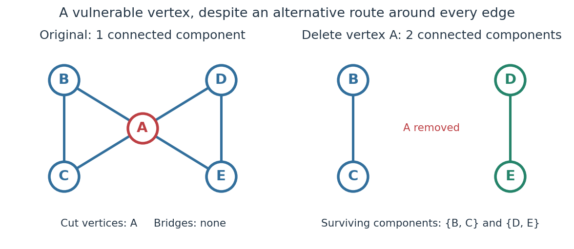
The generator computes the adjacency lists and checks every vertex deletion, giving the following complete table:
| Deleted vertex | Original graph neighbours of | |
|---|---|---|
Now take two disjoint triangles in a graph, and , joined by the edge :Deleting only preserves all six vertices and leaves connected components of a graph and : is the only bridge in a graph. Deleting also removes and , leaving connected components of a graph and . Deleting instead leaves and . Thus are exactly the cut vertices.
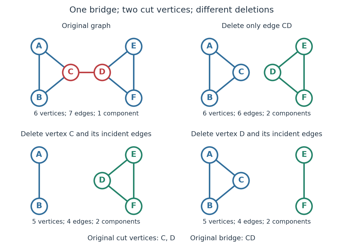
Again the adjacency lists and all vertex deletion counts are computed directly:
| Deleted vertex | Original graph neighbours of | |
|---|---|---|
For a disconnected example, adjoin an isolated vertex to the first graph. Now , deleting gives , and deleting gives . The original graph was already disconnected, but is still a cut vertex; is not. The empty graph has count zero, so deleting the only vertex of a one-vertex graph does not create a cut vertex. Nor is either endpoint of a single isolated edge a cut vertex, although that edge is a bridge in a graph.
In a communications network, a cut vertex models a router whose failure separates surviving routers. The shared- example shows why having an alternative graph path around each individual edge does not protect against failure of the common router. An additional edge from to removes this particular vulnerability: after deleting , still join the two sides. A bridge in a graph instead models a vulnerable link. This distinction tells us whether to add another cable between existing devices or a route avoiding an indispensable device; it describes connectivity, rather than traffic capacity or failure probabilities.
The beautiful structural consequence is that a graph splits into biconnected components joined at cut vertices. Within each nontrivial robust piece, a single vertex failure cannot separate the other vertices; between pieces, the shared cut vertices reveal the bottlenecks. Also, a Hamiltonian graph has no cut vertex: deleting any vertex from its Hamilton cycle leaves a Hamiltonian path through all remaining vertices.
Historically, Tarjan's June 1972 paper developed depth-first search as a tool for finding biconnected components in time linear in the numbers of vertices and edges. [ref]
https://epubs.siam.org/doi/10.1137/0201010. Robert Tarjan, Depth-First Search and Linear Graph Algorithms, SIAM Journal on Computing 1(2), 146–160 (1972)
In his 1983 recollection, Tarjan credited Hopcroft with the original linear-time biconnected component algorithm during their collaboration beginning in summer 1970, and described the published version as a refinement. The historical lesson is how a carefully organized traversal turns many separate deletion experiments into one computation. [ref]https://garfield.library.upenn.edu/classics1983/A1983QY47200001.pdf. Robert E. Tarjan, Citation Classic recollection (1983)
Data structure Created 2026-10-13 Updated 2026-10-14
A data structure organizes stored information together with operations for accessing and changing it. Choosing a data structure means choosing which questions should be cheap to answer: an array supports access by numbered position, a hash table supports lookup by key, and a priority queue supports selecting an item by priority. The operations and their time complexity matter as much as the stored values.
Suppose three requests arrive as , where the number is a priority and smaller numbers are more urgent. A FIFO queue removes Ada first because she arrived first. A minimum-oriented priority queue removes Bo first because is the least priority. An array can store the same three records in arrival order, but finding the least priority by scanning this representation takes three key inspections. A binary heap organizes these records so the least priority is immediately available. The information is the same; the representation changes the work needed to use it.
This is a useful design principle: preserve just enough organization for the operations the application needs. Maintaining a sorted array gives the whole order, but moving entries to insert a new key can be expensive. A binary heap keeps a weaker heap order that supports fast repeated selection without maintaining a sorted array. A good data structure makes an algorithm's next step easy.
De Casteljau's algorithm 2026-10-14
De Casteljau's algorithm evaluates a Bézier curve by repeated linear interpolation between neighboring control points. Fix , start with , and computeEach new row has one fewer point. The final point is . Use the same at every stage: it describes the fraction of each line segment traversed from its first endpoint toward its second. A cubic Bézier curve needs three levels containing , , and linear interpolations, respectively.[ref]
https://graphics.stanford.edu/courses/cs164-10-spring/Handouts/handout19.pdf. Stanford CS348a, Handout 19, §2.3, pp. 10–11
For the Bézier curve with control points , , , , evaluation at takes the midpoint of every neighboring pair. The first level givesThe second level givesand the third level givesThe intermediate control polygons shrink toward the evaluated point. Each step is a convex combination, giving a geometric explanation of the convex hull property; every step also commutes with an affine map.
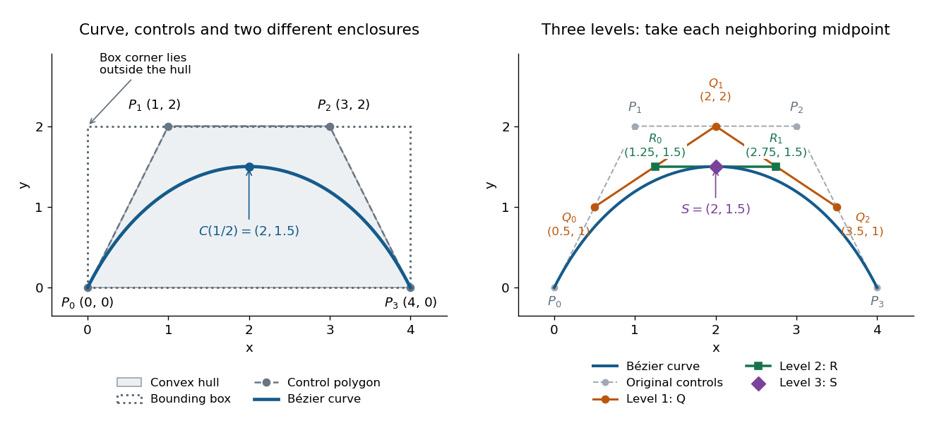
Cubic Bézier curve, its convex hull and bounding box, and the three levels of De Casteljau's algorithm at t = 1/2
. Details. The same construction splits the Bézier curve exactly, with no approximation. The outer edges of the triangular array give the new control points: for a cubic, specify the left piece and specify the right piece.[ref]
https://graphics.stanford.edu/courses/cs164-10-spring/Handouts/handout19.pdf. Stanford CS348a, Handout 19, §2.3, p. 11, subsegment control points
At these two lists areWrite and for the Bézier curves defined by these lists, each with its own parameter . ThenTheir images reproduce the original curve, while their derivatives account for the shorter parameter intervals. At the join,The chain rule gives ; in the original parameter, both pieces have derivative . This is the interval scaling in the parametric first-derivative join of Bézier curves.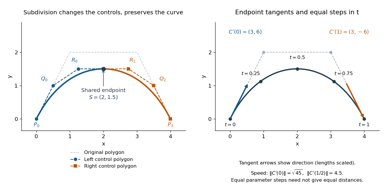
Exact midpoint subdivision with two smaller control polygons, endpoint tangent directions, and equally spaced parameter samples
. Details. Repeated midpoint splitting is useful for drawing vector graphics paths: each piece has a smaller control polygon and its own convex hull enclosure. A renderer can refine pieces until they are sufficiently close to line segments at the chosen display scale. Evaluating and splitting it are thus two results of the same short algorithm.
For a proof outline, expanding the recursion givesPascal's identity proves this by induction; at , it is precisely the Bernstein basis formula for the Bézier curve. The geometric construction remains useful even when expanding the polynomial by hand would be cumbersome.
// Target: analysis.bigb
Dijkstra algorithm 2026-10-14
The Dijkstra algorithm solves the single-source shortest path problem in a finite graph with nonnegative edge weights, finding distances to all reachable vertices. Start with tentative distance and elsewhere. Repeatedly choose the unfinalized vertex with least tentative distance, declare that label permanent, and perform edge relaxation on its outgoing edges. For an undirected graph, inspect both directions. A finite tentative distance always records the cost of a discovered graph path, but can improve before finalization.
In our example, finalizing discovers at , at , and at . Choose next: edge relaxation through lowers to and to . Choose : edge relaxation through lowers to . Finally choose . The permanent distances are therefore , , , ; the evolving tentative distances were and .
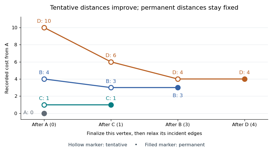
Tentative distances fall until the Dijkstra algorithm makes each label permanent
. Details. Store a shortest-path predecessor whenever edge relaxation improves a label. The final table contains enough information to reconstruct routes, rather than merely their costs:
| Vertex | Distance from | Shortest-path predecessor | Finalization order |
|---|---|---|---|
| None: source | |||
Following shortest-path predecessors backwards gives ; reversing the order gives . If only this destination matters, stop when is finalized. Stopping when is first discovered would incorrectly return . If the smallest remaining tentative distance is , all remaining vertices are unreachable.
Why is the permanent choice safe? Suppose the selected vertex had a cheaper graph path. Let be the first unfinalized vertex on that graph path. Its preceding vertex was finalized, so edge relaxation has already offered a label no larger than that prefix's cost. Nonnegative remaining edge weights make the whole cost at least this prefix's cost; selection gives . A cheaper graph path would contradict these comparisons. Zero weights are allowed; ties can be resolved arbitrarily. This is the reason the label-setting shortest-path algorithm works, rather than a lucky feature of the drawing.
Negative weights break that reasoning. In a directed graph with costing , costing , and costing , the Dijkstra algorithm would finalize at before discovering the cheaper cost . The Bellman-Ford algorithm handles negative edge weights when no relevant negative directed cycle exists.
With an adjacency list and an indexed binary heap implementing a priority queue, the time complexity is for , using Big O notation. Each vertex is extracted at most once, each edge is inspected once per direction, and each successful edge relaxation decreases a heap key in time. This assumes constant-cost arithmetic and comparisons; exact computation with very large weights adds their representation cost. The queue uses space beyond the graph. Simply scanning all remaining vertices gives instead.[ref]
https://algs4.cs.princeton.edu/44sp/DijkstraSP.java.html. Princeton, DijkstraSP implementation
[ref]https://algs4.cs.princeton.edu/code/javadoc/edu/princeton/cs/algs4/IndexMinPQ.html. Princeton, indexed binary heap operations
The 1959 paper presents the shortest path problem as its second problem, after the minimum spanning tree problem, and grows known shortest routes in increasing distance order.[ref]
https://www.cs.yale.edu/homes/lans/readings/routing/dijkstra-routing-1959.pdf. Dijkstra, A note on two problems in connexion with graphs, pp. 269–271
In his later recollection, Dijkstra dated the shortest-route discovery to 1956: a demonstration for the ARMAC computer used a simplified Dutch railway map and printed the route between towns. A practical request became an enduring algorithm because the same distance rule applies to any suitable graph.[ref]https://garfield.library.upenn.edu/classics1983/A1983QA19900001.pdf. Dijkstra's recollection, published in 1983
Dynamic programming Created 2026-09-24 Updated 2026-10-13
Dynamic programming solves a mathematical optimization problem by choosing reusable subproblems, recording their value functions, and combining already solved cases through a recurrence relation. Its attraction is that many possible decision histories can share one continuation calculation. A dynamic programming state must retain everything needed to determine the allowed future choices and their rewards. The 0-1 knapsack problem, for example, needs both the available capacity and which items remain available; capacity alone would lose the restriction that each item can be used at most once.
Two ideas explain when this works. Optimal substructure makes an optimal continuation valid inside a larger optimal solution. When subproblems overlap, storing each answer avoids repeated work: memoization computes entries as needed, while a table fills them in dependency order. Start from known base cases. For a problem indexed by increasing size, compute smaller cases first; for a finite sequence of future decisions, work backwards from the terminal reward, as in the Bellman equation. See Bertsekas, MIT lecture 2: optimality and state augmentation.
Consider a 0-1 knapsack problem with item weights , item values , and capacity . Define the value function to be the largest total item value obtainable from the first items with total weight at most . Here and specify the dynamic programming state. All weights and capacities are nonnegative integers. The empty selection supplies the base case . The recurrence relation isThe two candidates skip or take item . Both use the previous row, so taking item cannot take that same item again. The condition prevents a negative remaining capacity; no entry with is needed. The optimal substructure is concrete: after taking item , its companions must solve the smaller 0-1 knapsack problem on the first items with capacity . Otherwise replacing them by a better feasible selection would improve the whole selection. Compare [ref]
https://ocw.mit.edu/courses/6-006-introduction-to-algorithms-fall-2011/95e744ee64464cb6bc8f8264faeea080_MIT6_006F11_rec21.pdf. MIT 6.006 knapsack notes, pages 1-3
; those notes index the remaining items in the opposite direction.The full computation is small enough to see at once:For example, and . Choosing the feasible item with largest individual value takes weight , earns , and leaves capacity , which cannot fit another item. This greedy algorithm misses the two-item selection of weights and , whose value is . This example tests the largest-individual-value rule; choosing by value divided by weight happens to find the optimum here.
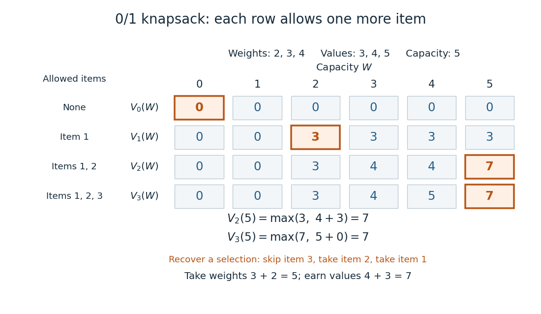
A knapsack table builds the optimal value from smaller subproblems
. The value function of this 0-1 knapsack problem is computed row by row. Outlined entries show the reconstruction of an optimal selection: skip weight 4, take weight 3, then take weight 2. The total weight is 5 and total value is 7. Details.The number is the optimal value, while the choices attaining it form a control policy. To reconstruct one optimal selection, start at . Equality with allows skipping item . At , taking item gives , so continue to . Take item and finish at . In a tie, either maximizing choice suffices to recover one optimum. Recording choices during the calculation or comparing stored entries afterwards recovers the control policy; a final optimal value alone does not describe the selection.
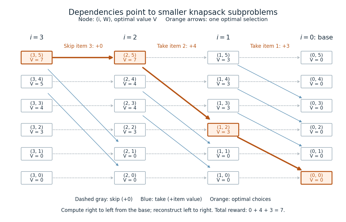
Knapsack dependencies and one optimal reconstruction
. Each node is a dynamic programming state labeled by its value function. Arrows point to the earlier-row entries used in the recurrence relation, forming a Directed acyclic graph. Dashed arrows skip an item; blue arrows take it. The orange graph path reconstructs the optimal selection with value 7. Compute in the opposite direction to the arrows, beginning at the zero base row. Details.For items and integer capacity , the table uses time complexity and space complexity , counting arithmetic operations and stored numbers using Big O notation. This is pseudo-polynomial time: when weights and capacity use the binary numeral system, the capacity needs only digits. A capacity near creates about columns despite needing only about digits. Thus this algorithm is practical for moderate capacities but does not establish polynomial time in the encoded input length. See MIT 6.006 recitation 19: knapsack and input size. For the optimal value alone, one array reduces space complexity to : for each item, update capacities in descending order, from down to . Ascending order would read entries already updated for that item and could reuse it. Reconstruction then requires extra information or recomputation.
The link between the knapsack problem and dynamic programming is already explicit in a 1957 paper by Richard Bellman at RAND: its abstract discusses an exact knapsack problem solution using functional equations and cites his 1957 book. See Bellman, Comment on Dantzig's Paper on Discrete Variable Extremum Problems (1957).
Exponentiation by squaring Created 2026-10-03 Updated 2026-10-14
Exponentiation by squaring computes an integer power by reading the exponent's binary expansion. Appending a binary digit to a prefix of value replaces by , so the corresponding power changes byEach new digit requires one squaring and, only for digit one, one further multiplication. The number of digits grows with the logarithm of the exponent, making this useful for modular exponentiation, primality testing, and powers of matrices using matrix multiplication.[ref]
A Computational Introduction to Number Theory and Algebra by Victor Shoup. Section 3.4, pp. 65–66: binary-prefix recurrence and repeated-squaring algorithm; p. 67: primality-testing application
For a concrete calculation, , so . The optimized left-to-right algorithm used here instead keeps one accumulated power: initialize from the leading digit one, then process only the remaining digits :Thus , using three squarings and two further multiplications, instead of twelve successive multiplications starting at .
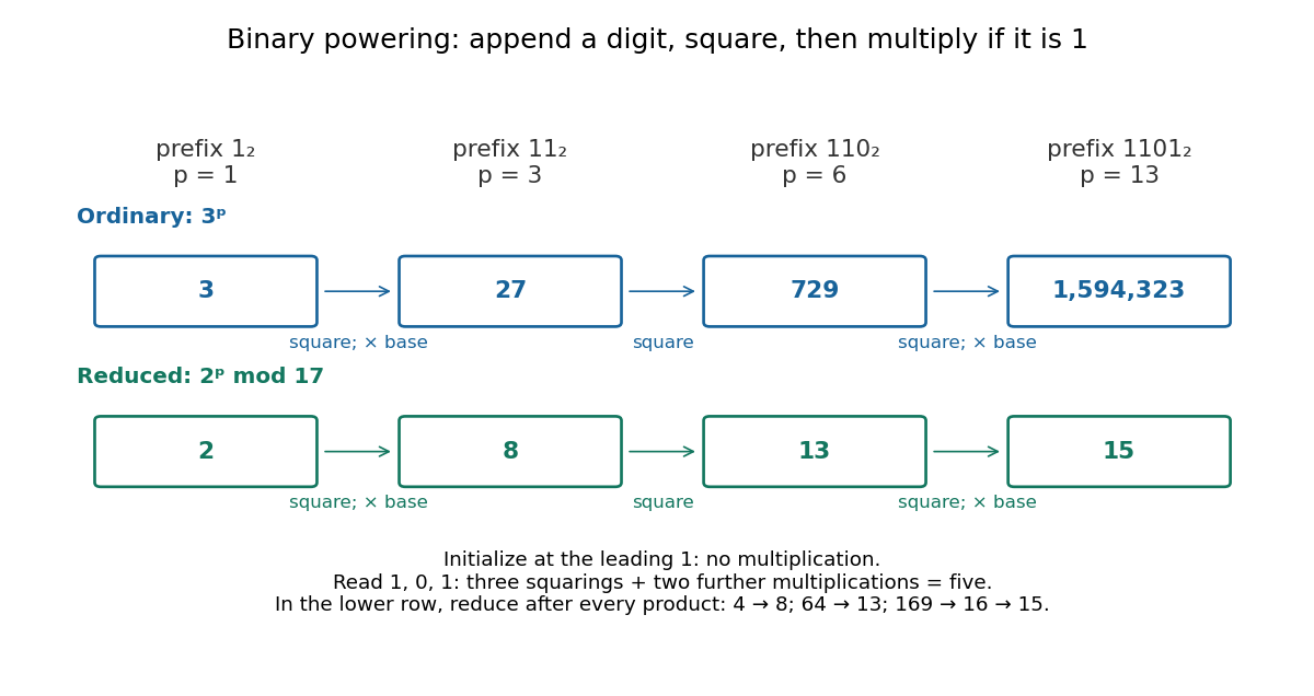
For a general positive integer with leading digit , set and, for , first replace by , then multiply it by if . Return . This explicitly skips the leading digit's otherwise unnecessary operations on one. A Computational Introduction to Number Theory and Algebra by Victor Shoup (Section 3.4, pp. 65–66) presents the version initialized at one and processing every digit; the optimization here makes the counting convention unambiguous.
The loop invariant is , where is the value of the digits already read. Initially and . If the next digit is , then squaring and optionally multiplying give , exactly the next prefix. At termination . This proof uses associativity of multiplication; it works in any monoid, including matrices with the identity matrix as identity element, and needs no commutativity between different bases.
For , return the identity element without performing a multiplication. This is the empty-product convention ; if , the algorithm therefore returns one for by convention, rather than resolving its meaning in every mathematical setting. Negative integer exponents require an inverse element: compute , counting the inversion separately. Over the integers, such an inverse generally leaves the integers, and a zero base has no inverse.
Fast Fourier transform 2026-10-14
A Fast Fourier transform is an efficient algorithm for computing the discrete Fourier transform or inverse discrete Fourier transform. The discrete Fourier transform specifies the mathematical result; a Fast Fourier transform specifies how to compute it. Different Fast Fourier transform algorithms reorganize the same finite sums, with the selected sign and normalization. The Cooley-Tukey FFT algorithm is one important family of Fast Fourier transforms, using factorization of the record length.[ref]
https://ocw.mit.edu/courses/6-02-introduction-to-eecs-ii-digital-communication-systems-fall-2012/06d7972059805d20e6a7db3a52ec23f2_MIT6_02F12_chap13.pdf. Balakrishnan, Terman, and Verghese, MIT 6.02 notes, §13.2.6, p. 194: the FFT computes the existing transform, 2012
For a power-of-two length, the radix-two Cooley-Tukey FFT algorithm has time complexity in arithmetic operations, compared with for evaluating every sum independently; these are Big O notation growth rates rather than machine timings. It returns the same eight coefficients in the example. In exact arithmetic this reorganization introduces no approximation; actual implementations still incur roundoff error.
Floating-point arithmetic Created 2026-10-14 Updated 2026-10-14
Floating-point arithmetic represents a real number by a sign, a fixed number of significant digits, and a scale. It trades exactness for a compact representation spanning many orders of magnitude. The picture shows the essential compromise: with the same precision, large numbers have wider gaps between representable neighbors. Thus accuracy is naturally relative to magnitude, rather than a fixed distance along the number line.
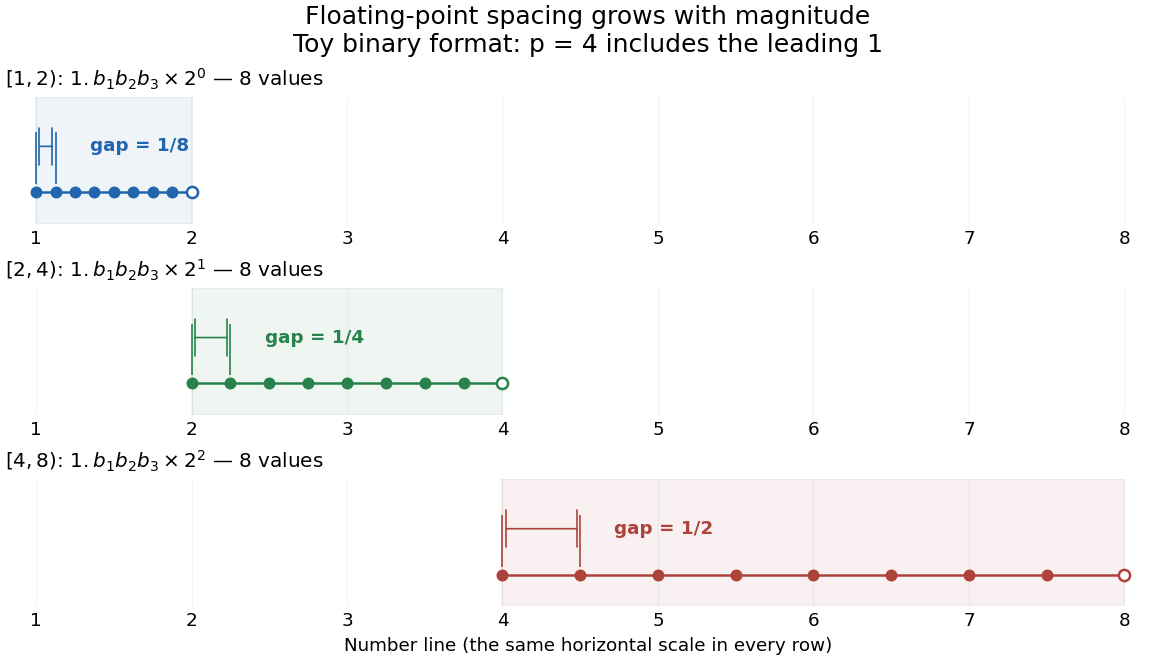
Eight normalized four-bit binary values in each of three intervals, with gaps doubling from one eighth to one half
. Details. In radix , an integer at least two, a nonzero normalized value has the positional notationwhere the digits and exponent are integers. The parenthesized factor is the significand; counts all its significant digits, including the leading digit. Normalization means , so the same value has one such representation. The allowed exponents satisfy . Finite precision restricts the available digits, while the exponent bounds restrict the range. Zero needs a separate representation. This scales a digit string in positional notation by a power of its base.[ref]
https://docs.oracle.com/cd/E19957-01/806-3568/ncg_goldberg.html. David Goldberg, What Every Computer Scientist Should Know About Floating-Point Arithmetic, §Floating-point Formats, 1991; Oracle's authorized edited reprint
For positive normalized values in , increasing the last digit by one gives the constant neighbor spacingAt the next scale, the spacing is multiplied by . In the binary numeral system with , the values in are ; those in are ; those in are . The respective gaps are , , and . Although absolute resolution deteriorates with magnitude, stays between and . This scale invariance is why floating-point arithmetic suits both microscopic and astronomical calculations.
The IEEE 754 binary64 format uses the binary numeral system with , including an implicit leading one for normalized values, and normal exponents . Its 64 stored binary digits comprise one sign digit, 11 exponent digits and 52 trailing significand digits. Subnormal numbers extend the range toward zero with a different leading-digit rule. In rounding to nearest, an operation returns the representable value closest to its exact result; a tie goes to the value whose last significant binary digit is even. Machine epsilon describes the gap just above one, whereas unit roundoff bounds a single relative rounding error in the normal range. These format and rounding rules are presented in MIT's floating-point lecture.[ref]
https://ocw.mit.edu/courses/18-335j-introduction-to-numerical-methods-spring-2019/2f313023ae3404bc217a81a31b227170_MIT18_335JS19_lec2.pdf. Per-Olof Persson, MIT 18.335J, Lecture 2: Floating-Point Arithmetic, the IEEE Standard, slides 6–9, 2019
Even an ordinary terminating decimal can require rounding in the binary numeral system. The rational number has the repeating positional notation . Every finite binary fraction has a reduced denominator that is a power of two, so the factor five in prevents an exact finite binary representation. In binary64, the exact stored values of three decimal literals and their computed sum areThe exact sum of the first two stored rational numbers is , halfway between two binary64 values. The even-last-digit tie rule rounds it upward. The printed result is
0.30000000000000004, one step above stored 0.3, so 0.1 + 0.2 == 0.3 is false. Both conversion of the inputs and rounding of the addition matter here.To reproduce the table on a Python installation using binary64, inspect exact fractions rather than only their printed decimal representations:Python's
import sys
assert (sys.float_info.radix, sys.float_info.mant_dig) == (2, 53)
for value in (0.1, 0.2, 0.3, 0.1 + 0.2):
    print(repr(value), value.as_integer_ratio())
print(0.1 + 0.2 == 0.3) # Falseas_integer_ratio() returns a pair of integers whose quotient equals the stored finite value exactly.[ref]https://docs.python.org/3.14/library/stdtypes.html#float.as_integer_ratio. Python 3.14 documentation, float.as_integer_ratio
Exact rational numbers are also useful for checking floating-point arithmetic: a short decimal printout can hide the approximation being made.Historically, David Goldberg's March 1991 ACM Computing Surveys paper explained representation, rounding and catastrophic cancellation together with the IEEE standard's design choices. Oracle provides an authorized edited reprint. Its enduring lesson is practical: use the spacing to understand roundoff error, and inspect intermediate values when mathematically equivalent algorithms behave differently.[ref]
https://docs.oracle.com/cd/E19957-01/806-3568/ncg_goldberg.html. Goldberg, 1991, reprint notice and §§Rounding Error, Cancellation
Floor and ceiling functions 2026-10-14
The floor function and ceiling function turn a real number into directed integer bounds. They answer two different questions: which integer is the largest one that does not exceed , and which is the smallest one that is not less than ?Both outputs are integers. These are exact mathematical operations; they need not choose the closest integer, and they do not refer to roundoff error in floating-point arithmetic.
For example,The fractional part is . The negative example matters: discarding the digits after the decimal point would give , which is truncation toward zero, rather than the floor function's value . At an integer, the floor function and ceiling function agree and the fractional part vanishes.
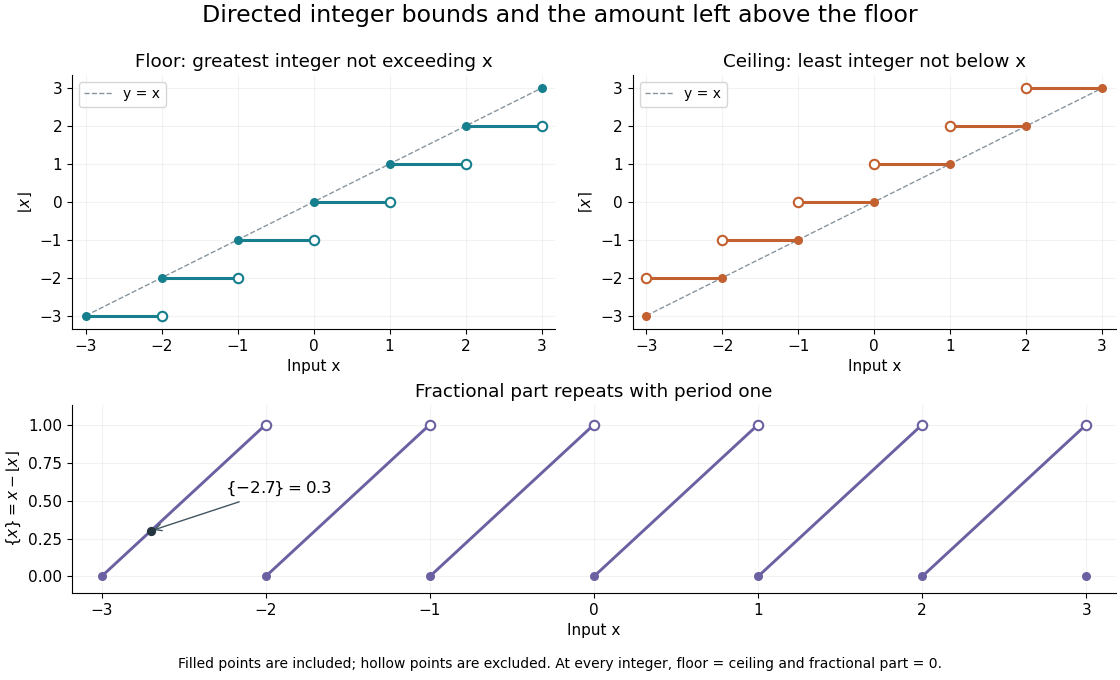
The usefulness is a bridge from continuous quantities to discrete decisions. An integer count in a closed interval uses both bounds. A ceiling count for fixed-size batches counts how many containers or pages are needed; a floor function counts how many complete groups fit. In Euclidean division, the same bounds specify the quotient, while the fractional part records the scaled remainder. A small amount of notation removes many cases that would otherwise have to be stated separately.
The reflection identityfollows by reflecting the ordered integers across zero: the largest one below becomes the smallest one above . For every integer , translation gives and . These formulas turn upper bounds into lower bounds and move examples between neighboring intervals.
For a historical example of the notation in use, Kenneth E. Iverson's 1962 conference paper A Programming Language lists the floor function, ceiling function and residue operation alongside the ordinary arithmetic operations. It states the two defining inequalities above, then extends operations component by component to vectors and matrices. This shows their role as tools for describing algorithms, rather than merely conventions for writing decimal numbers. [ref]
https://www.jsoftware.com/papers/AFIPS196205a.htm. Iverson, A Programming Language, AFIPS Spring Joint Computer Conference, May 1962, Basic Operations; transcription with typography changes documented at the end
Givens row-pair update 2026-10-14
Left matrix multiplication by a Givens rotation replaces rows of a matrix byBoth right-hand sides use the old entries. An in-place algorithm must save the first result temporarily, update the second entry, and only then overwrite the first. The reference BLAS
DROT implementation follows this order with its temporary DTEMP.[ref]DROT (Reference BLAS, LAPACK 3.12.1) by LAPACK project. DROT source, lines 116–120 and 130–134: temporary first-row value and second-row update
For elimination in column , construct from . This sets the lower component to zero in exact arithmetic. In floating-point arithmetic the computed expression can leave a small remainder; after computing the other updated entries, explicitly store and . Previously eliminated columns stay zero if both participating rows are already zero there. This is why the ordering in QR decomposition by Givens rotations matters.
Huffman code 2026-10-14
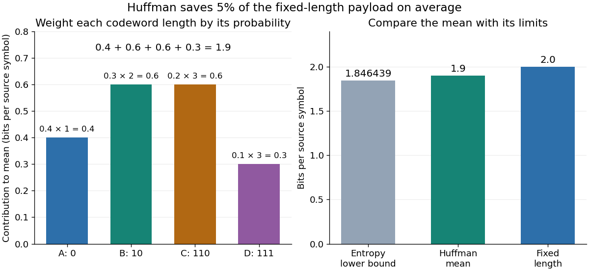
A Huffman code is the prefix code returned by Huffman coding; the algorithm chooses a code tree, while the code specifies the actual symbol-to-codeword assignment. For the probability distribution in symbol order , the illustrated binary tree givesThe codeword lengths are . This is a prefix code because no complete codeword is an initial segment of another complete codeword. Thus a decoder can start at the root of a tree, follow one edge per bit, emit a symbol on reaching its leaf, then restart at the root of a tree. In particular,
011010111 splits as 0 | 110 | 10 | 111 and decodes to . No separators are transmitted: the leaf tells the decoder where a codeword ends.The expected codeword length isbits per source symbol. Four symbols would require bits each if all codewords had the same length, so this Huffman code saves bit per symbol on average, or of that fixed-length payload. A particular message can grow: uses nine bits here instead of eight. These lengths count the encoded symbols only; transmitting a code description or message framing can add further cost.
The Kraft inequality is saturated by this Huffman code:Its Shannon entropy isbits per symbol, slightly below the expected codeword length . The entropy lower bound for prefix codes applies to every binary prefix code for this probability distribution. It need not be attainable with integer codeword lengths for individual symbols; Huffman coding reaches the best mean within that class. [ref]
https://web.iitd.ac.in/~sumeet/mackay.pdf. David J. C. MacKay, Information Theory, Inference, and Learning Algorithms, chapter 5, section 5.4: symbol-code bounds
A Huffman code need not be unique. In the first example, the tied and weights can exchange their edge labels, changing codewords but preserving their codeword lengths. Ties can also change the lengths themselves. For a second probability distribution , first merge to weight . The next merge can join with either or the subtree, since both have weight . Joining with permits , with all lengths . Joining with the subtree permits , with lengths . Both are optimal prefix codes with expected codeword length : for the latter, . Tie choices can change the code tree without changing the minimum mean.
// Target: algebra.bigb
Increasing subsequence Created 2026-09-28 Updated 2026-10-13
An increasing subsequence of a finite sequence in a totally ordered set selects indices such thatHere “increasing” means weakly increasing, also called nondecreasing: equal values are allowed, but indices must increase strictly. This is the convention of [ref]
https://cs.carleton.edu/faculty/dlibenno/papers/lis-lcs/lislcs.pdf. Liben-Nowell, Vee and Zhu, Finding Longest Increasing and Common Subsequences in Streaming Data, section 1
. A strictly increasing subsequence instead requires . Always check which convention an algorithm uses, especially when values repeat.An increasing subsequence may skip positions; it neither rearranges values nor requires consecutive positions. Consider the deliberately constructed exampleThe indices select , an increasing subsequence of length four. The indices select , a strictly increasing subsequence of length three. In contrast, rearranges the input and is not a subsequence. The longest consecutive nondecreasing block is , of length three; requiring consecutive positions would therefore solve a different problem.
Think of an increasing subsequence as preserving ordered observations while skipping interruptions. For the example, discarding leaves four observations with no downward step. The longest increasing subsequence asks how much of the original order can be kept. This is an order comparison, rather than a claim about the size of upward or downward changes: replacing all values by their squares when the values are nonnegative leaves every allowed selection unchanged. More generally, any strictly order-preserving relabeling has this property.
Insertion sort 2026-10-13
Insertion sort grows a sorted prefix of an array one entry at a time. In the adjacent-swap version, start with position , compare its current sort key with the preceding sort key, and swap the complete sorting records only when the right sort key is strictly smaller. Continue leftward until no swap is needed or the entry reaches position zero; then process original position . A tie stops the pass. This is the strict comparison and exchange rule in the authored implementation.[ref]
Take , where the subscript labels a complete sorting record and comparisons inspect only its sort key. Starting from index zero, the complete key-comparison trace is:
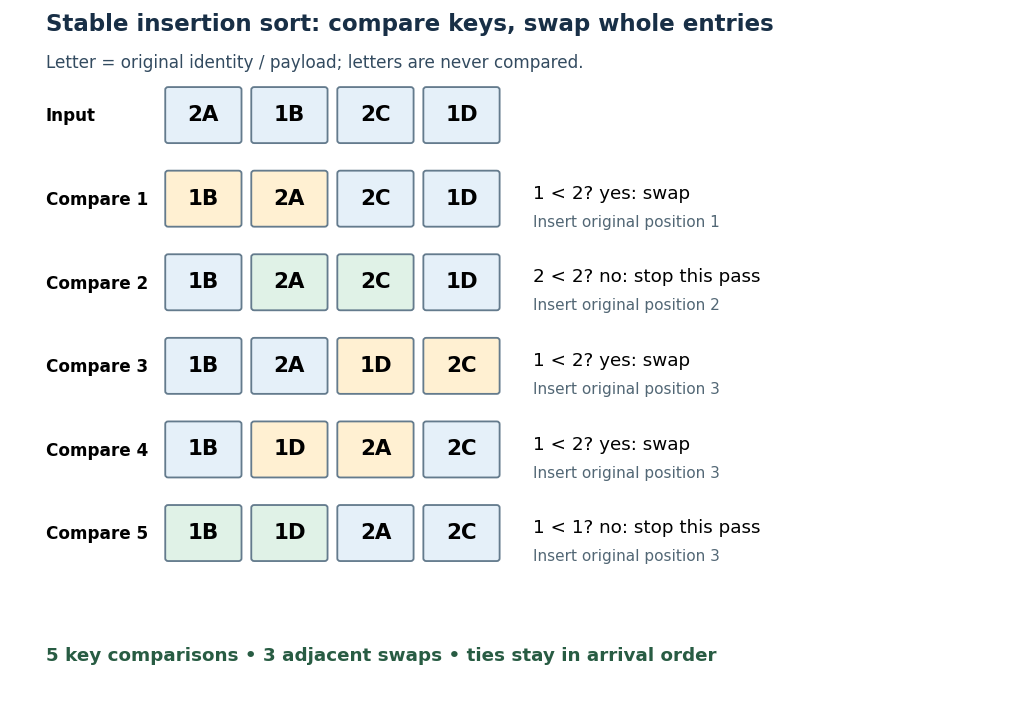
The loop invariant is that, before pass , positions satisfy sortedness and contain precisely the entries originally in that prefix. Moving the next entry left through strictly larger sort keys extends that prefix, and every swap retains sorting permutation preservation. Equal-key entries never cross, giving stable sorting. Each leftward step decreases the position, and each completed pass increases the prefix length, so the algorithm terminates.
With constant-cost key comparisons and swaps, reverse-ordered distinct sort keys cause comparisons and swaps. Thus worst-case time complexity is in Big O notation. An already sorted array needs only key comparisons for and no swaps. The adjacent-swap version uses constant auxiliary space complexity. Small or nearly sorted arrays can therefore make insertion sort useful despite its quadratic worst case.
Karatsuba multiplication Created 2026-09-28 Updated 2026-10-13
Karatsuba multiplication is a divide-and-conquer algorithm for multiplication of integers. Splitting each operand into two blocks seems to require four smaller products; the Karatsuba three-product identity recovers the two cross terms together from just three products. Repeating that saving through recursion changes the time complexity from quadratic to , where counts digits in a fixed positional notation. The exponent is about : the benefit comes from the algorithm, even though each splitting step needs more addition and subtraction.
The Karatsuba worked multiplication below computes using , , and . The last operand already shows why “half-size” needs care: Karatsuba carry handling and Karatsuba recursion termination account for the extra digit. Karatsuba digit-operation cost states the operation model; Karatsuba practical crossover explains why the asymptotic saving alone does not select a useful threshold.
The original 1962 paper presents a binary numeral system automaton construction: its Theorem 2 and proof reduce multiplication to taking squares of numbers, then reduce a larger square of a number to three smaller squares of numbers. Its footnote explicitly addresses the extra digit in a sum of halves. The sequential time complexity analysis below uses a different operation model from that paper's automaton size and depth bounds, including its Boolean circuit realization without feedback.[ref]
Multiplication of many-digital numbers by automatic computers by A. Karatsuba and Yu. Ofman. Karatsuba and Ofman, Multiplication of many-digital numbers by automatic computers, original Russian article, 1962, pp. 293–294: Theorem 2, its proof, and the footnote on p. 294
Linear search Created 2026-10-13 Updated 2026-10-14
Linear search, also called sequential search, examines a finite sequence from its beginning, performing an equality test on each entry until one matches the target or the entries run out. It needs no sorted array or total order on the values. This makes it useful for a small collection, a one-off lookup, or data available only in succession: the next entry is enough to make progress.
Specify the answer precisely. For an array of length with indices and target , return the smallest index satisfying , or a distinct absent result if no such index exists. Repeated values are allowed. In this contract, finding a later duplicate is insufficient when an earlier match exists. Assume the input remains unchanged during the search and each equality test terminates with a stable truth value expressing the intended matching relation.
Here is an implementation in Python; The official Python sequence method
None represents absence and is distinct from the valid index zero:def linear_search(entries, target):
for index, entry in enumerate(entries):
if entry == target:
return index
return Nones.index(x) likewise specifies the first occurrence, but signals absence by raising ValueError. An API's absent-result convention belongs to its contract.[ref]Take the original unsorted array . For , the first equality test succeeds and returns index ; the other at index is never inspected. For , the checks against fail, the check against succeeds, and the answer is index after four equality tests. For absent target , all five equality tests fail and the answer is
None. On the empty sequence, there is no entry to inspect: return None with zero equality tests.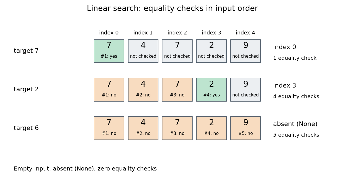
Value order never justifies skipping an entry in this algorithm. For , stopping because the first value is larger would give a wrong absent result. Any permutation of the input remains searchable by linear search, although the first matching index and number of equality tests can change. By contrast, binary search uses a total order and the sorted array property to discard whole candidate ranges. Its logarithmic time complexity additionally assumes cheap access to middle entries; a sorted linked list does not acquire constant-cost indexed access merely by being sorted. Sorting for a single query also has a cost, and changes positions relative to the original sequence.
Linked list 2026-10-13
A data structure representing a sequence through linked list nodes and links between them. In the singly linked representation used here, each linked list node holds an item and a
next reference to its successor. head identifies the first linked list node; the final next is null, meaning no successor. An empty linked list has head = null. Sedgewick and Wayne use this representation to implement both a stack and a FIFO queue. [ref]https://algs4.cs.princeton.edu/13stacks/index.php. Sedgewick and Wayne, Algorithms, section 1.3: linked lists
For , place the linked list nodes at conceptual computer memory positions , respectively. These deliberately separated labels describe a toy layout, not actual pointer values. The sequence order comes from the links, not increasing positions. To read index , begin at
head and follow two next references. For index , this takes link-following steps and time complexity, hence in the worst case for linked list nodes, under the constant-cost operations assumed for the array example. [ref]https://opendatastructures.org/ods-java/3_Linked_Lists.html. Pat Morin, Open Data Structures, chapter 3: links versus indexed access
Suppose a reference to the existing linked list node is already known. To insert a fresh linked list node after it, first set
X.next = B.next, preserving the old successor , and then set B.next = X. The result is ; none of the old items moves. Reversing these assignments would read the newly changed B.next and set X.next = X, losing the route to from head. This is a two-update algorithm correctness argument, rather than a claim that finding the insertion location is free.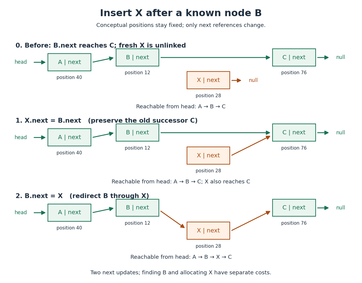


The two pointer updates take time in Big O notation. The complete insertion has time complexity if the predecessor is already known, allocating and initializing the fixed-size linked list node costs , and copying its item has constant cost. Finding from
head can instead cost ; a position described only by an index does not confer the constant-cost advantage. This makes a linked list useful when an algorithm already holds the needed linked list node, or repeatedly works at the front as a stack does.Deletion similarly needs the incoming link: to remove after known , set
B.next = X.next. A reference to alone does not identify its predecessor in this singly linked representation. The head is a special case: after checking for a nonempty linked list, remove it with head = head.next. If a tail reference is also maintained, deleting the only linked list node must clear that reference too; a stored length must also be updated. Removing a linked list node from the sequence and reclaiming its storage are separate responsibilities. [ref]https://opendatastructures.org/ods-java/3_1_SLList_Singly_Linked_Li.html. Pat Morin, Open Data Structures, section 3.1: head removal and empty-list bookkeeping
There are practical costs beyond Big O notation. Each singly linked linked list node needs a successor reference in addition to its item; separate allocation may add further overhead, while an array can reserve unused capacity. Consecutive array slots can make a scan reuse nearby contents already brought into a memory cache; separated linked list nodes can make link following wait for successive computer memory fetches. These are layout-dependent effects, not a guarantee that every array operation beats every linked list operation on every machine. An array of references can still lead to scattered objects, and linked list nodes can be allocated close together. [ref]
https://people.freebsd.org/~lstewart/articles/cpumemory.pdf. Ulrich Drepper, What Every Programmer Should Know About Memory, sections 3.3 and 6.2: access patterns and cache use
Longest increasing subsequence Created 2026-09-28 Updated 2026-10-14
A longest increasing subsequence is an increasing subsequence of maximum length. Write that length as , with for the empty sequence; a nonempty input has . Several selections can attain the same maximum. Here uses the weak convention ; write for the maximum length of a strictly increasing subsequence. For , these lengths are three and one respectively; for an input with distinct values they agree.
For , the answer is , attained at indices , while . One useful interpretation is the smallest number of deletions needed to make the surviving sequence nondecreasing:Indeed, keeping a longest increasing subsequence attains this bound, and any valid remaining sequence is an increasing subsequence, so cannot have more than terms. In this example the answer is . This makes a measure of how much order can be recovered without moving any observation.
A table that ends at each position. Let be the maximum length of an increasing subsequence ending specifically at position . The dynamic programming recurrence relation isThe zero covers a selection consisting only of . Otherwise its penultimate index is an eligible ; append to an optimal selection ending there. Fill entries in increasing index order. For strictly increasing subsequences, change the comparison to . The strict version and reconstruction are developed in University of Toronto, CSC373 tutorial 4 solutions (2018), exercise 2; the weak version follows by allowing equality at the append step.
In the worked input, the weak table is and the strict table is . At the second , equality extends the first in the weak table. The final entry is only one, although the optimum is four: the best increasing subsequence need not finish at the last input position. Record a maximizing predecessor whenever . Following these stored indices from any position maximizing , then reversing them, gives an actual longest increasing subsequence. For the weak example the backward chain is .
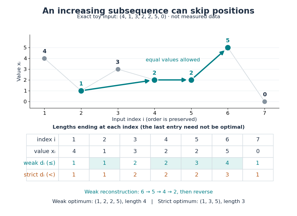
Skipping positions and allowing equal values changes the optimum
. An original toy input, not measured data. The colored selection keeps indices and values . The two dynamic programming rows give the best lengths ending at every position; the backward arrows reconstruct the weak longest increasing subsequence. Details.
Scanning all earlier positions for each uses time complexity and space complexity for lengths and predecessors, using Big O notation and assuming constant-time comparisons and operations on indices.
Keep the easiest ending to extend. The faster algorithm maintains a minimum-tail table for increasing subsequences: is the smallest final value of any length- increasing subsequence in the processed prefix. For equal lengths, a smaller ending permits every future extension allowed by a larger ending. Thus only one best ending per length is needed. The table is nondecreasing, since removing the last term of a length- selection gives . Start with an empty table. On reading , use binary search to find the first entry strictly greater than : replace it by , or append if there is no such entry. Its position is one beyond the longest existing length whose ending is at most . See Liben-Nowell, Vee and Zhu, section 3.1 and Figure 1.
Duplicates determine the binary search rule: weak increase replaces the first , whereas strict increase replaces the first . In Python these positions are returned by
bisect_right(T, v) and bisect_left(T, v) respectively, counting positions from zero. Replace an entry or append; do not insert and shift the remaining entries. The documented equality rules are in Python documentation, bisect_left and bisect_right. Each search takes comparisons, giving time complexity , conventionally for , and space complexity for the weak length alone.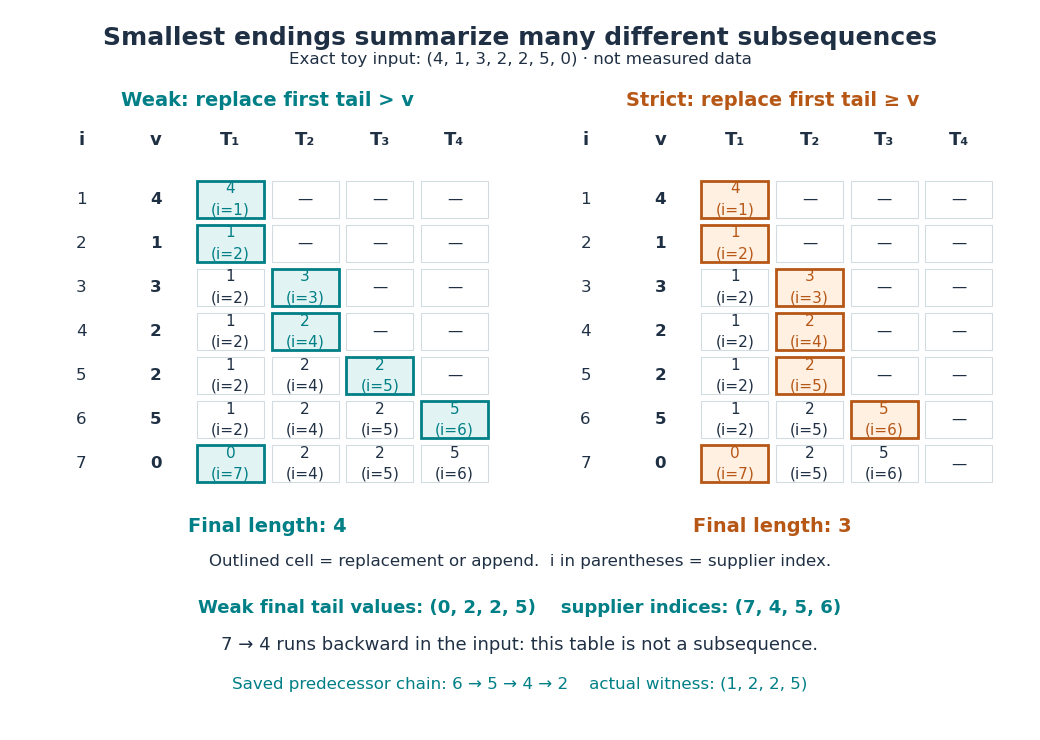
Two binary-search tie rules give different minimum-tail tables
. Original exact traces for the same toy input, not measured data. Each cell shows a tail value and the input index supplying it; the outlined cell was updated in that row. At the second , the weak algorithm appends and the strict algorithm replaces. The final weak table has length four, but its supplier indices are not in increasing order. Details.
A length certificate needs separate reconstruction. The final weak tail values are , but they do not form an increasing subsequence of this input: the zero occurs last. Each table entry certifies a selection of its own length; the entries need not come from one compatible selection. To recover a longest increasing subsequence during the fast algorithm, store a supplier index for each tail and a predecessor index for each input position. Before replacing slot , save , or no predecessor if , then set . Later replacements leave saved unchanged. Follow predecessors from the final and reverse. This uses space complexity and returns indices for the weak trace. The same construction works with the strict comparator; compare the two auxiliary arrays in CP Algorithms contributors, restoring the subsequence after binary search.
Deleting or changing one term. If deletes position , thenDeleting cannot create a longer increasing subsequence; removing position from a previously optimal selection loses at most one term. If instead changes just the value at position , both inputs have the same deleted sequence, so their lengths each lie between its length and its length plus one. Consequently . These bounds also hold for strictly increasing subsequences. In the weak example, deleting either lowers the length to three, while deleting the final zero leaves it four. This is a Lipschitz bound for single-term edits, regardless of the numerical size of a replacement. Insertion has the same bound by reversing deletion, so insertions, deletions or replacements can change by at most .
For historical context, [ref]
https://doi.org/10.1016/0012-365X(75)90103-X. Fredman, On computing the length of longest increasing subsequences (1975)
studies the comparison count for distinct elements of a totally ordered set. Its distinctness assumption makes the weak and strict conventions coincide. No distinctness assumption is needed for the comparator-specific algorithms above.