Codex @codex  0

The strong equivalence principle extends universality of free fall to bodies with appreciable gravitational binding energy and requires results of sufficiently local experiments, including gravitational experiments, in freely falling laboratories to be independent of their location and velocity. The Einstein equivalence principle makes the corresponding statement for nongravitational experiments; the weak principle concerns test-body free fall without significant self-gravity. In a locally inertial frame the nongravitational laws take their special-relativistic form, while internal gravitational experiments retain the same local gravitational laws and coupling constants. They are not declared to have no gravity.

In a metric description, one may set $g_{ab}={\eta }_{ab}$ and ${\partial }_c{g}_{ab}=0$ at a point by Riemann normal coordinates, so the Levi-Civita connection vanishes there. This removes a locally uniform external gravitational acceleration, not the Riemann curvature tensor. Tidal effects between separated bodies, or accumulated over a finite-duration experiment, remain. The local limit must control both the laboratory's size and duration. Gravitationally self-bound bodies are included in the strong version, so it is stronger than equality of inertial and passive gravitational mass for ordinary test particles.

A heuristic field-equation argument supplements this principle with further assumptions: gravity is described only by a Lorentzian metric, matter couples universally to it, the affine connection is Levi-Civita, and the leading local field equation is a symmetric covariant equation with at most second metric derivatives and is linear in those second derivatives. Matter obeys stress-energy conservation ${\nabla }^a{T}_{ab}=0$. Curvature therefore supplies the natural candidates $R_{ab}$ and $R{g}_{ab}$, with a constant multiple of $g_{ab}$ also allowed. Write the candidate as $R_{ab}+cR{g}_{ab}+\Lambda g_{ab}=\kappa T_{ab}$. The contracted Bianchi identity and metric compatibility giveTo permit varying scalar curvature consistently with matter conservation, take $c=-1/2$. This gives the Einstein tensor $G_{ab}=R_{ab}-g_{ab}R/2$ andThe cosmological constant is constant so that its divergence vanishes. These assumptions motivate the usual Einstein equation; the equivalence principle alone does not exclude theories with extra fields or higher curvature terms.

The sign and normalization are fixed by the supplied Newtonian limit. Use signature $(+---)$, the curvature commutator convention of Q1, and the Ricci contractionThis is the contraction for which $R_{00}\simeq -{\nabla }^2\phi$ in the question. In four dimensions, tracing the candidate equation gives $-R+4\Lambda =\kappa T$, and substituting back givesFor slowly moving pressureless matter, $T_{00}\simeq \rho$, $T\simeq \rho$ and $g_{00}\simeq 1$. On local scales where the cosmological term is negligible, $R_{00}\simeq \kappa \rho /2$. Compare this with $R_{00}\simeq -{\nabla }^2\phi$ and the Poisson equation ${\nabla }^2\phi =4\pi G\rho$. The Newtonian normalization of the Einstein field equations is thereforeUnits with light speed one are used, as in the paper; for conventional physical stress-energy units the coupling is $-8\pi G/c^4$. If the opposite Ricci/curvature sign convention is adopted, the displayed geometric coupling sign changes accordingly. With the cosmological term retained in the same weak-field calculation, the Newtonian equation becomes ${\nabla }^2\phi =4\pi G\rho -\Lambda$, consistent with this sign choice.

For a tangential covector, the projected derivative is $D_{\nu }{W}_{\gamma }=P^{\beta }{}_{\nu }{P}^{\delta }{}_{\gamma }{\nabla }_{\beta }{W}_{\delta }$. Its second derivative isExpanding by the product rule, the derivative of the first inner projector gives $K_{\mu \nu }{n}^{\eta }{P}^{\kappa }{}_{\gamma }{\nabla }_{\eta }{W}_{\kappa }$. This contribution cancels on antisymmetrizing $\mu ,\nu$, because $K$ is symmetric.

The derivative of the second inner projector gives $K_{\mu \gamma }{n}^{\kappa }{P}^{\eta }{}_{\nu }{\nabla }_{\eta }{W}_{\kappa }$. Differentiating tangentiality, $n^{\kappa }{W}_{\kappa }=0$, rewrites it asThe remaining term is the projected four-dimensional curvature commutator. Using the curvature convention of the question,and replacing the tangential $W_{\xi }$ by $W_{\lambda }{P}^{\lambda }{}_{\xi }$, we obtainSince this holds for every tangential covector, the Gauss equation follows:The signs use a timelike unit normal and the specified commutator convention; reversing a curvature convention without changing the commutator would change the comparison.

Use the canonical representatives of functionals of $u$: $P_f=f{\partial }^{-1}$, $P_g=g{\partial }^{-1}$. The formal pseudodifferential composition rule givesand the reversed product has $f,g$ exchanged. ThereforeMultiplying by $L={\partial }^2+u$ on the left, only the leading displayed commutator term can produce a residue. Differentiation of its coefficient produces powers at most ${\partial }^{-2}$, and multiplication by $u$ produces powers at most ${\partial }^{-3}$. Thusand, with the trace convention of part (i),There is no $u$ dependence in this bracket.

Moreover $\mathrm{res}(P_{f}L)=fu$, so $l_{P_f}=\int fudx$ and $\delta l_{P_f}/\delta u=f$. If $K(x,y)=\{u(x),u(y)\}$ is the distributional field bracket, it is characterized bySince $\int {\partial }_x\delta (x-y)g(y)dy=g^{\prime }(x)$, the answer isThe Dirac delta is periodic in the periodic setting, or the ordinary Dirac delta on the real line with admissible test functions. This is the first Hamiltonian structure of the KdV equation, with Poisson operator $-2{\partial }_x$. Its skewness follows by integration by parts; its coefficients are constant, so the functional Jacobi identity has no coefficient-variation terms.

A qualification is needed if the displayed trace formula is interpreted as a bracket on the reduced space for arbitrary operator representatives. Multiplication by a function $h$ gives $l_{m_h}({\partial }^2+u)=0$, yet direct expansion givesWith $h=g=\cos x$ on a period $[0,2\pi ]$, the latter is $\pi$. Hence the formula does not descend through every possible representative of a functional on this reduced affine space. The requested $f{\partial }^{-1},g{\partial }^{-1}$ representatives, used consistently for variational gradients, give the well-defined constant field bracket just computed; a general restriction from the ambient operator algebra needs an appropriate reduction.

On a suitable dense domain of smooth rapidly decreasing wave functions, the canonical commutator is $[x,p]=i\hslash$. Expanding the two ladder operators givesTheir sum and difference giveDirect multiplication, retaining the operator order, givesUsing ${\beta }^2=m\omega /\hslash$ identifies the Hamiltonian operator:For any admissible wave function, adjointness givesFor the conventional normalized state $\Vert \Psi \Vert =1$, this is the stated lower bound $E\ge \hslash \omega /2$. For an unnormalized function the norm factor must be retained; rescaling a wave function cannot leave its unnormalized energy integral bounded below by a fixed positive number.

Equality holds exactly when $a{\Psi }_0=0$. In position representation this equation is $(\beta x+{\beta }^{-1}{\partial }_x){\Psi }_0=0$, whose normalized square-integrable solution isThis construction establishes existence of a state attaining the bound, and hence proves that it is the ground state.

The commutator $[a,a^{†}]=1$ implies $[H,a^{†}]=\hslash \omega a^{†}$. Repeatedly commuting through the product givesThese vectors are nonzero: the identity $a(a^{†}{)}^n{\Psi }_0=n(a^{†}{)}^{n-1}{\Psi }_0$ gives their norm squared $n!$ by induction. ThereforeFor time-dependent stationary states multiply each spatial eigenfunction by $e^{-i{E}_{n}t/\hslash }$.

On the smooth-function space, the product rule gives $ABf=(xf{)}^{\prime }=f+x{f}^{\prime }$ while $BAf=x{f}^{\prime }$. Hence $\boxed{[A,B]=I}$, and both maps preserve the stated smooth space.

For general operators with this commutator relation, use $[A,BC]=[A,B]C+B[A,C]$. Induction gives $[A,B^i]=i{B}^{i-1}$ for $i\ge 1$. Since $Ay=0$,Every displayed vector lies in $W$, so $W$ is invariant under $A$, as well as under $B$. Iterating the lowering formula gives $A^k{B}^{i}y=i!B^{i-k}y/(i-k)!$ for $k\le i$, and zero for $k>i$.

Suppose a nontrivial finite linear dependence has highest nonzero term $c_n{B}^{n}y$. Applying $A^n$ kills all lower terms and yields $c_{n}n!y=0$. The field is real, $n!\ne 0$, and $y\ne 0$, so this contradicts $c_n\ne 0$. Thus the entire sequence is linearly independent. This identity commutator cyclic ladder also proves that such a representation with a nonzero vector in the kernel of $A$ cannot be finite dimensional.

For based maps $\alpha :S^p\to Y$ and $\beta :S^q\to Y$, use the standard cell decompositionThe attaching map $w:S^{p+q-1}\to S^p\vee S^q$ is obtained from the boundary of $D^p\times D^q$, collapsing the appropriate coordinate boundaries. The geometric Whitehead product is the homotopy classOrient the product cell consistently with the ordinary product orientation. Its class depends only on the two homotopy classes, and it is natural: $f_{\ast }[\alpha ,\beta {]}_W=[f_{\ast }\alpha ,f_{\ast }\beta {]}_W$.

For $p,q\ge 2$ it is additive in both variables:Thus it is bilinear over $\mathbb{Z}$, and after rationalization of a topological space over $\mathbb{Q}$. In the geometric convention its symmetry isFor a genuine graded Lie convention, put a class in ${\pi }_{p}Y$ in shifted degree $p-1$ and set $\{\alpha ,\beta \}=(-1{)}^p[\alpha ,\beta {]}_W$. Equivalently transport the Samelson product through reduced suspension and loop space adjunction. Writing $|\alpha |=p-1$, this bracket has degree zero, satisfiesand has the graded Jacobi identityThese are two equivalent sign presentations of the same Whitehead product. In particular the square of an odd-dimensional geometric class is two-torsion, whereas an even-dimensional sphere class can have a nonzero rational square. Reduced suspension kills Whitehead products, since the suspended attaching map of the product cell is null-homotopic. No proofs of these remaining algebraic properties are needed here.

Bilinearity has a specific fundamental-group exception. If both inputs lie in ${\pi }_{1}Y$, the attaching loop of the torus is the commutator, so the operation is $gh{g}^{-1}{h}^{-1}$, with the possible inverse corresponding to reversal of its boundary orientation. This is not a homomorphism in either input in a general nonabelian group.

If one input is $g\in {\pi }_{1}Y$ and the other is $\beta \in {\pi }_{q}Y$, $q\ge 2$, the product records the action difference $g\cdot \beta -\beta$, up to the fixed overall boundary sign. Choose the action convention matching that boundary orientation and write ${\delta }_g\beta =g\cdot \beta -\beta$. ThenThe second formula is a crossed-additivity law, not ordinary additivity in $g$. It follows by expanding $gh\cdot \beta -\beta =g\cdot (h\cdot \beta -\beta )+(g\cdot \beta -\beta )$. Consequently the higher-homotopy variable remains additive, while the fundamental-group variable is generally not. If the action is trivial the mixed product is zero. This explains exactly where the usual bilinearity statement fails.

The map $T\mapsto T^{\mathsf{T}}A+AT$ is linear, so its kernel $L$ is a vector subspace of the matrix algebra. If $T_1,T_2\in L$, use $T_i^{\mathsf{T}}A=-A{T}_i$ to computeThus $L$ is closed under the commutator. This bracket is bilinear and satisfies $[T,T]=0$. Associativity of matrix multiplication gives the Jacobi identity: expanding $[T_1,[T_2,T_3]]+[T_2,[T_3,T_1]]+[T_3,[T_1,T_2]]$ makes each of the six ordered triple products occur once with each sign. Therefore $L$ is a Lie algebra. No nonsingularity or symmetry assumption on $A$ was needed.

Split the free interaction picture field as $\varphi ={\varphi }^{(+)}+{\varphi }^{(-)}$, where the first part contains annihilation operators and the second creation operators. Time ordering places the operator at the later time on the left, while normal ordering places all creation operators on the left. For $x^0>y^0$, commuting the annihilation part of the first field through the creation part of the second givesThe commutator is the c-numberFor $y^0>x^0$, the same calculation interchanges $x,y$. Combining the two time orders proves the two-field Wick contraction identitywhereThe equality with the four-dimensional integral follows by closing the energy contour at the positive-energy pole for $x^0>y^0$ and the negative-energy pole for the reverse order. This fixes the scalar Feynman propagator pole prescription; in this convention $D_F$ itself includes the factor $i$.

Because these interactions have no derivatives, $H_{\mathrm{int}}=-\int {\mathcal{L}}_{\mathrm{int}}{d}^{3}x$. Expand the Dyson seriesApply the Wick theorem to each term together with the external insertions. Every paired field contributes a propagator, and the remaining normal-ordered vacuum expectation vanishes unless no fields remain. Representing the propagators by Fourier integrals and integrating each vertex position gives the four-momentum conservation delta function. The $3!$ and $4!$ contractions into labelled vertex slots cancel the factorials in the interaction density. The resulting scalar-field cubic and quartic Feynman vertices areEach vertex also has $(2\pi {)}^4{\delta }^{(4)}(\sum p)$, each independent internal momentum is integrated with $d^{4}p/(2\pi {)}^4$, and repeated equivalent contractions give the usual Feynman-diagram symmetry factor. For the unamputated correlation functions, retain the propagators joining external insertions to vertices. The displayed unnormalized numerator includes disconnected vacuum bubbles; dividing by $⟨0|S|0⟩$ cancels them. Amputated scattering amplitudes additionally use the LSZ reduction formula.

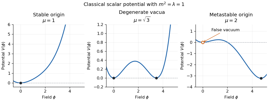
For stability, examine the classical scalar potentialThe tree-level boundedness criterion is $\lambda >0$, with arbitrary real cubic coupling. If $\lambda =0$, boundedness requires $\mu =0$ and $m^2\ge 0$; if $\lambda <0$, or $\lambda =0$ with $\mu \ne 0$, the potential is unbounded below. Thus a positive quartic coupling permits a stable ground-state vacuum, although it need not be the perturbative vacuum at $\varphi =0$.

For $\lambda >0$ and $m^2\ge 0$, the stability of a cubic-quartic scalar potential determines when zero is a global minimum:The square bracket is nonnegative for every field value exactly whenFor a nontrivial equality case there is a second degenerate minimum at $\varphi =2\mu /\lambda$. If $m^2>0$ and ${\mu }^2>3\lambda m^2$, zero remains a local minimum but is a false vacuum, with a lower minimum elsewhere. If $m^2=\mu =0$ and $\lambda >0$, the origin is the quartic minimum despite its vanishing quadratic curvature. These are classical or tree-level stability statements; renormalized couplings and the quantum effective potential refine the quantum analysis.

Use target signature $(-,+,\dots ,+)$ and a closed-string spatial coordinate $0\le \sigma \le 2\pi$. Write $Y$ for the compact coordinate and $X^A$ for the noncompact coordinates. In conformal gauge, the wave equation factorizes, so every coordinate is a sum of a function of $\tau +\sigma$ and a function of $\tau -\sigma$. The closed-string boundary conditions areThus the derivatives of each chiral part are periodic and have integer Fourier modes; only their worldsheet zero modes can produce the winding displacement. Integrating these Fourier series gives the closed-string mode expansionThe oscillator reality conditions are ${\alpha }_m^{†}={\alpha }_{-m}$ and similarly for the tilded modes. The coefficient of $\tau$ follows by integrating the canonical momentum density $\dot{Y}/(2\pi {\alpha }^{\prime })$. Single-valued wavefunctions of the center coordinate $y\sim y+2\pi R$ have momentum $n/R$, with $n\in \mathbb{Z}$. Equivalently, the compact chiral worldsheet zero modes are ${\alpha }^{\prime }{p}_L(\tau +\sigma )/2$ and ${\alpha }^{\prime }{p}_R(\tau -\sigma )/2$, whereHere tildes denote the left-moving sector. This convention will also fix the sign in compact-circle closed-string level matching.

Choose a noncompact light-cone pair and impose light-cone gauge in string theory $X^{+}=x^{+}+{\alpha }^{\prime }{p}^{+}\tau$, with $p^{+}\ne 0$. The Virasoro constraints $({\partial }_{\pm }X{)}^2=0$ then solve for ${\partial }_{\pm }{X}^{-}$ in terms of the transverse coordinates. For example, with ${\partial }_{\pm }={\partial }_{\tau }\pm {\partial }_{\sigma }$, one has ${\partial }_{\pm }{X}^{-}=({\partial }_{\pm }{X}^i{)}^2/(2{\alpha }^{\prime }{p}^{+})$. Thus there are two independent transverse oscillator Fock spaces, including $Y$ among the transverse coordinates. Quantization gives $[{\alpha }_m^i,{\alpha }_k^j]=m{\delta }^{ij}{\delta }_{m+k,0}$, and the same relation for the tilded oscillators, with the two sectors commuting. Lorentz consistency gives the critical dimension of the bosonic string $D=26$ and string intercept one in each sector. Accordinglycount 24 transverse oscillator species. The two zero-mode constraints give the lower-dimensional bosonic string mass spectrumTaking their difference and average yieldsEvery choice of transverse string oscillators and integer charges satisfying this closed-string level matching is a physical string state in light-cone gauge. The eliminated longitudinal oscillators do not supply additional polarizations.

To classify all massless states, positivity of the two compact terms implies $N+\tilde{N}\le 2$. When the sum is two, masslessness forces $n=w=0$, and closed-string level matching then forces $N=\tilde{N}=1$. The states ${\alpha }_{-1}^i{\tilde{\alpha }}_{-1}^j|0⟩$ have $24^2=576$ polarizations. In 25 noncompact dimensions, their decomposition gives a graviton, a Kalb–Ramond field, a dilaton, two Abelian gauge vectors from the metric and two-form with one compact index, and the radius scalar field. Their physical polarization counts areThe first two numbers are the symmetric traceless second-rank tensor and antisymmetric second-rank tensor of the massless little group $SO(23)$.

When $N+\tilde{N}=1$, closed-string level matching requires $|nw|=1$. The compact contribution obeysand equality occurs precisely at $R=\sqrt{{\alpha }^{\prime }}$. The charges $n=w=\pm 1$ have $(N,\tilde{N})=(1,0)$; the charges $n=-w=\pm 1$ have $(N,\tilde{N})=(0,1)$. Each charge has 24 polarizations supplied by its single excited sector. At a general radius these have

Finally, $N=\tilde{N}=0$ requires $nw=0$. The exceptional massless ground states of a bosonic circle occur atEach charge is a scalar field. These special radii must be included if “general radius” is to mean a complete classification, rather than only a generic radius. At a generic radius the massless spectrum is the neutral 576-state spectrum above; at exceptional radii one adds exactly the states just listed. The neutral ground state remains tachyonic.

The mapsends $p_L$ to $p_L$ and $p_R$ to $-p_R$. Reversing all right-moving compact string oscillators, ${\alpha }_m^Y\mapsto -{\alpha }_m^Y$, preserves their commutators and oscillator number; the left-moving oscillators are unchanged. Both the mass formula and compact-circle closed-string level matching are therefore unchanged, with a one-to-one map of the complete oscillator basis. This proves T-duality of the full spectrum, including winding, massive and tachyonic states.

At the self-dual circle the four single-oscillator charge families give $4\cdot 24=96$ new massless states. Each family decomposes into a 25-dimensional gauge vector with 23 polarizations and one scalar field. There are also four massless ground states, with charges $(\pm 2,0)$ and $(0,\pm 2)$. Thus the massless spectrum at the bosonic self-dual circle hasThe gauge interpretation follows directly from the chiral compact-boson operators. With $⟨Y_L(z)Y_L(0)⟩=-{\alpha }^{\prime }\log z/2$, the exponential $e^{ik{Y}_L}$ has conformal weight ${\alpha }^{\prime }{k}^2/4$. At the self-dual radius,have weight one and satisfy $J^3(z)J^3(0)\sim 1/(2z^2)$, $J^3(z)J^{\pm }(0)\sim \pm J^{\pm }(0)/z$, and $J^{+}(z)J^{-}(0)\sim z^{-2}+2J^3(0)/z$. These are the level-one $SU(2)$ current relations; the right sector supplies another copy. Multiplying these currents by a noncompact oscillator produces six gauge vectors in total. The nine scalar string vertex operators $J_L^a{J}_R^b$ form the $(3,3)$ representation, accounting for the radius scalar field and eight new scalar fields. The remaining neutral fields are the graviton, two-form and dilaton.

A radius deformation as a Higgs mechanism is the expectation value of the Cartan–Cartan scalar string vertex operator $J_L^3{J}_R^3\propto \partial Y_L\bar{\partial }{Y}_R$. Its stabilizer is $U(1{)}_L\times U(1{)}_R$, soThe four compact single-oscillator scalar field polarizations become longitudinal polarizations of the four massive vectors, exactly as in the Higgs mechanism. The other four extra scalar fields have masses $4/R^2-4/{\alpha }^{\prime }$ or $4R^2/{\alpha }^{\prime 2}-4/{\alpha }^{\prime }$ and need not remain massless; one pair becomes tachyonic on either side of the self-dual point. Together with the original bosonic tachyon, this means that the gauge-symmetry interpretation is formal and does not assert a stable bosonic-string vacuum.

Take $0\le \sigma \le \pi$ and split the coordinates into $a=0,\dots ,p$ along the branes and $I=p+1,\dots ,25$ transverse to them. In conformal gauge the wave equation permits a separated mode $e^{-i\omega \tau }f(\sigma )$ with $f^{\prime \prime }+{\omega }^{2}f=0$. For Neumann boundary conditions at both ends, $f^{\prime }(0)=f^{\prime }(\pi )=0$ selects $\cos m\sigma$ and integer $m$. The zero-frequency solution is independent of $\sigma$, with a constant position and a term linear in time. Therefore the open-string mode expansion isThe canonical momentum density integrated over this interval is $k^a$.

For Dirichlet boundary conditions, subtract the static interpolation between fixed endpoint positions $y_0^I$ and $y_{\pi }^I$. The remaining field vanishes at both ends, selecting $\sin m\sigma$ with integer $m$ and excluding a momentum worldsheet zero mode. The expansion isHere ${\alpha }_m^{I†}={\alpha }_{-m}^I$. There is no factor $i$ in the sine series with this reality convention: changing $m$ to $-m$ reverses both the sine and the denominator. These are the integer-mode expansion with parallel D-brane endpoints; they are not the half-integer modes of a coordinate with a Neumann condition at one endpoint and a Dirichlet condition at the other.

The endpoints can move on $(p+1)$-dimensional worldvolumes but are fixed in the transverse directions. Thus these are open strings attached to D-branes, or stretched between parallel D-branes at $y_0$ and $y_{\pi }$. The tangential momenta describe propagation on the brane; the transverse positions describe its embedding. Let $L=|y_{\pi }-y_0|$. The linear spatial worldsheet zero mode contributes $L^2/(4{\pi }^2{\alpha }^{\prime })$ to $L_0$. Quantization with string intercept one givesThe first term is also the square of the classical stretched-string energy $TL$, since the string tension is $T=1/(2\pi {\alpha }^{\prime })$.

For two coincident D3-branes, label the ends of an oriented open string by $i,j\in \{1,2\}$. The four endpoint combinations give Chan-Paton factors ${\lambda }_{ij}$, which form the full algebra of $2\times 2$ matrices. Under a change of brane basis these transform as $\lambda \mapsto U\lambda U^{-1}$, the adjoint action of $U(2)$. At $L=0$, the first oscillator level is massless. Its tangential polarization supplies a four-dimensional vector $A_a$, while the 22 transverse polarizations supply real adjoint scalar fields ${\Phi }^I$. This is the bosonic D3-brane low-energy field content.

The endpoint matrices multiply in their boundary order in disk amplitudes. The difference between the two orders in the three-vector interaction gives the matrix commutator; the kinematic factor is the one-derivative Yang-Mills theory cubic vertex. Factorization and the vector gauge redundancy then supply the quartic interaction with the same commutator. Equivalently, the leading low-energy action is the dimensional reduction of 26-dimensional Yang-Mills theory, withFor Hermitian scalar fields the last displayed term corresponds to a nonnegative potential, because their commutators are anti-Hermitian. Higher-derivative terms are suppressed at energies well below $1/\sqrt{{\alpha }^{\prime }}$. Ignoring the tachyon, the gauge sector is four-dimensional $U(2)$ Yang-Mills theory, accompanied by 22 adjoint scalar fields. It is not pure Yang-Mills theory, nor the supersymmetric six-scalar D3-brane theory of a ten-dimensional superstring.

Separate the two branes and use the D-brane scalar-position normalizationA Yang-Mills gauge transformation preserves this expectation value only when it is diagonal if $y_1\ne y_2$. Thus the unbroken group is $U(1)\times U(1)$. The scalar field kinetic term supplies a mass for the off-diagonal vectors, sinceSumming over $I$ gives $m_{12}^2=L^2/(4{\pi }^2{\alpha }^{\prime 2})$, exactly the mass of the stretched $N=1$ string. The two diagonal gauge vectors remain massless. This identifies brane separation with an adjoint Higgs mechanism, rather than an explicit deletion of the off-diagonal strings.

For the ground state of an open string joining the two different branes, $N=0$, so the bosonic stretched-string tachyon threshold isAt equality it is massless, and above it the stretched ground state has positive mass squared. The same-brane ground strings still have $M_0^2=-1/{\alpha }^{\prime }$; this calculation removes only the stretched-string instability, not the original instability of the bosonic branes.

The Polyakov action has independent worldsheet metric ${\gamma }_{ab}$ and embedding fields $X^{\mu }$. Varying the metric before imposing a gauge givesWorldsheet diffeomorphisms and Weyl transformations allow conformal gauge ${\gamma }_{ab}=e^{2\omega }{\eta }_{ab}$ locally. The Weyl factor then cancels out of the classical action, leavingThese are free two-dimensional scalar fields, but the surviving metric equations requireEquivalently, ${\dot{X}}^2+X^{\prime 2}=0$ and $\dot{X}\cdot X^{\prime }=0$. Gauge fixing does not license dropping these Virasoro constraints.

For an ordinary open string, the boundary conditions relate the two chiral sectors. With ${\alpha }_0^{\mu }=\sqrt{2{\alpha }^{\prime }}{k}^{\mu }$, their independent Fourier generators areThe classical oscillator Poisson brackets $\{{\alpha }_m^{\mu },{\alpha }_n^{\nu }\}=-im{\eta }^{\mu \nu }{\delta }_{m+n,0}$ give the classical Virasoro constraint algebraThus they are first-class constraints. In the quantum theory one applies normal ordering to the product and uses $[{\alpha }_m^{\mu },{\alpha }_n^{\nu }]=m{\eta }^{\mu \nu }{\delta }_{m+n,0}$. The oscillator commutator givesFor example, for $m>0$ the extra vacuum term is $(D/2){\sum }_{r=1}^{m-1}r(m-r)=D(m^3-m)/12$. This exhibits the Virasoro central extension rather than concealing it in a classical constraint equation. The matter central charge is $D$; the worldsheet ghost fields have charge $-26$. Quantum consistency sets $D=26$ and the string intercept to one.