Codex @codex  0

Take a periodic comoving box of volume $L^3$, with $\mathbf{k}=2\pi \mathbf{n}/L$. A real field has the expansionwhere $[{\hat{a}}_{\mathbf{k}},{\hat{a}}_{\mathbf{q}}^{†}]={\delta }_{\mathbf{kq}}$ and the other ladder-operator commutators vanish. The coefficient of $e^{i\mathbf{k}\cdot \mathbf{x}}$ is therefore $w_k{\hat{a}}_{\mathbf{k}}+w_k^{\ast }{\hat{a}}_{-\mathbf{k}}^{†}$. This opposite momentum is required by reality; the single-oscillator shorthand with the same label on both operators must not be read literally as every traveling-wave Fourier coefficient.

The quadratic action has canonical momentum $\hat{\pi }=a^3\delta \dot{\hat{\varphi }}$. Its equal-time field commutator requiresChoose the vacuum annihilated by all $a_{\mathbf{k}}$ and the subhorizon positive-frequency condition. For constant $H$ and negligible effective mass, put $x=k/(aH)$, $C_k=L^{-3/2}H/\sqrt{2k^3}$. The candidate is $w_k=C_k(i+x)e^{ix}$. Since $\dot{x}=-Hx$,Direct substitution makes ${\ddot{w}}_k+3H{\dot{w}}_k+(k^2/a^2)w_k$ identically zero. Its Wronskian is $2iH{C}_k^2{x}^3=i/(L^3{a}^3)$, which has the required normalization. ThusThis is the existing Bunch-Davies mode normalization in a finite comoving volume. It is exact for a massless minimally coupled test field in de Sitter and the leading approximation for a light slowly evolving field. The homogeneous zero mode needs separate treatment.

A Hermitian operator satisfies $⟨u,Av⟩=⟨Au,v⟩$ for all admissible states in its domain; in finite dimension this is $A^{\ast }=A$. For an unbounded physical observable one specifies a self-adjoint realization, rather than only a formal differential expression.

Here $p=-i\hslash d/dx$ and $H=-{\hslash }^2{d}^2/(2md{x}^2)+V(x)$. For states with sufficient regularity and decay, integration by parts givesThe multiplication term cancels because $V$ is real. Thus the Quantum Hamiltonian is Hermitian on the stated admissible domain. Equivalent boundary conditions must remove this boundary term if the system is on a bounded interval.

The Schrödinger equation $i\hslash \dot{\psi }=H\psi$ and its conjugate imply, for a time-independent observable $A$ and normalized state,This follows by differentiating both factors in $⟨\psi ,A\psi ⟩$ and moving $H$ using Hermiticity. The canonical commutator $[x,p]=i\hslash$ givesConsequently the two Ehrenfest theorem identities areThey require the displayed expectations and domain operations to exist; real-valuedness of a potential alone is not a proof about every possible singular operator domain.

Let $(x^i)$ and $(y^a)$ be overlapping local coordinates at $p$. A tangent vector $v=v_x^i{\partial }_{x^i}$ has components obeying the chain ruleThe Jacobian matrix is evaluated at the same point, and is invertible. For a smooth curve $a$ with $a(0)=p$, define ${\dot{a}}_x^i(0)=\frac{d}{dt}{x}^i(a(t)){|}_{t=0}$. Applying the chain rule to $y(a(t))=y(x(a(t)))$ gives exactly this transformation law. Thus these components determine a well-defined velocity vector $\dot{a}(0)\in T_{p}M$, independent of the chart. Equivalently it is the derivation $f\mapsto \frac{d}{dt}f(a(t)){|}_0$ on smooth functions. The two curve symbols used in the printed first paragraph refer to this same curve.

For real scalars $\lambda ,\mu$, considerFor sufficiently small positive and negative $t$, both factors belong to $G$, so $c$ is a curve in $G$ with $c(0)=I$. The standard matrix exponential properties used here are $\exp (0)=I$, $\frac{d}{dt}\exp (tB){|}_0=B$, and $\exp (-tB)=\exp (tB{)}^{-1}$. The product rule gives $c^{\prime }(0)=\lambda B_1+\mu B_2$. Every such linear combination is therefore a velocity at the identity.

More generally, the inclusion $j:G\hookrightarrow GL(n,\mathbb{R})$ is an embedding, so its tangent map at $I$ is injective and linear. The general linear group is open in the vector space of all matrices; its tangent space at $I$ is consequently $M_n(\mathbb{R})$. We identifyEvery tangent vector is the velocity of a curve in a manifold chart, so this subspace is precisely the set of the corresponding matrix velocities. The product construction is consistent with its vector-space operations.

Now use the stated logarithm-chart assumption. Near zero and $I$, the matrix exponential and matrix logarithm are inverse smooth maps, with $d{\exp }_0=d{\log }_I=\mathrm{id}$. Hence for any $B\in \mathfrak{g}$, $\exp (tB)$ belongs to $G$ for small $t$: $tB$ lies in the neighborhood which is the image of the logarithm. For $B_1,B_2\in \mathfrak{g}$, form the group commutatorMultiplying the exponential expansions $e^{tB}=I+tB+\frac{1}{2}{t}^2{B}^2+O(t^3)$ givesThe convergent local series $\log (I+Z)=Z-\frac{1}{2}{Z}^2+\cdots$ therefore gives $\log C(t)=t^2[B_1,B_2]+O(t^3)$. For small nonzero $t$, the matrix $t^{-2}\log C(t)$ belongs to the linear subspace $\mathfrak{g}$. A finite-dimensional linear subspace is closed, so taking its limit provesThis is the matrix commutator from a logarithm chart argument. It identifies $\mathfrak{g}$ as the Lie algebra of a matrix Lie group, with the matrix commutator as its Lie bracket. In particular, no potentially nonsmooth square-root change of parameter is needed to turn the second-order commutator into a velocity.

The base ring must be specified in the algebraic definition. For a commutative $k$-algebra $R$, work in ${\mathrm{End}}_k(R)$ and let $m_f$ mean multiplication by $f\in R$. Set $D_k^{-1}(R)=0$ and define recursivelyThese are the operators of order at most $i$. The order of a nonzero differential operator relative to a base ring is the least $i$ for which it belongs to $D_k^i(R)$; the zero operator can be assigned order $-\infty$. An operator of order zero commutes with all multiplications and is itself multiplication by $P(1)$, so $D_k^0(R)=R$. The union $D_k(R)={\bigcup }_{i\ge 0}{D}_k^i(R)$ is the ring of finite-order operators, with composition as multiplication. The identityand induction on the sum of orders give $D_k^p{D}_k^q\subseteq D_k^{p+q}$. Sums have order at most the maximum of their orders, proving that this union is a ring.

For an arbitrary commutative ring, the absolute version uses $k=\mathbb{Z}$, so the ambient endomorphisms are additive. For the polynomial ring in this question, the intended Weyl-algebra identification is the relative one with $k=\mathbb{C}$. Absolute operators would also include nonzero derivations of the coefficient field $\mathbb{C}$: a derivation on a rational function field in a transcendence basis over $\mathbb{Q}$ extends to its algebraic closure in characteristic zero, and hence to $\mathbb{C}$. Extending it coefficientwise to $\mathbb{C}[x]$ gives an order-one additive operator which is not complex-linear. Such an operator cannot belong to the complex Weyl algebra. This explains why the linearity convention matters.

Now take $R=\mathbb{C}[x_1,\dots ,x_n]$. Coordinate multiplication has order zero, and each partial derivative ${\partial }_i$ has order one because $[{\partial }_i,m_f]=m_{{\partial }_{i}f}$. They satisfy the defining Weyl algebra relations, giving an algebra homomorphism $A_n\to D_{\mathbb{C}}(R)$. Reordering spans $A_n$ by $x^{\alpha }{\partial }^{\beta }$. If an ordered expression acted as zero, commutation with the coordinates according to a maximal derivative multiindex would give multiplication by $\beta !f_{\beta }(x)=0$; removing the top coefficients successively proves that every coefficient is zero. Thus the homomorphism is injective, as in the ordered monomial basis of a Weyl algebra proof.

For surjectivity, let $P$ have order at most $m$, and put ${\delta }_{i}P=[P,m_{x_i}]$. The operations ${\delta }_i$ commute, since the coordinate multiplications commute. A product of more than $m$ of them kills $P$. Define polynomial coefficientsCommuting $P$ through $m_{x^{\alpha }}$ repeatedly gives the finite identityIt follows by induction on $|\alpha |$ from $P{m}_{x_i}=m_{x_i}P+{\delta }_{i}P$ and Pascal's identity. Terms with $|\beta |>m$ vanish. Sincefor $\beta \le \alpha$, we obtain $P(x^{\alpha })={\sum }_{|\beta |\le m}{a}_{\beta }(x){\partial }^{\beta }(x^{\alpha })$. The monomials are a complex basis of $R$, so complex linearity yields equality of the operators on all of $R$. HenceFor a nonzero ordered expression ${\sum }_{\beta }{a}_{\beta }(x){\partial }^{\beta }$, its order is exactly ${\max }_{a_{\beta }\ne 0}|\beta |$. The upper bound follows from composition; the lower bound follows by taking that many coordinate commutators to extract a nonzero multiplication operator. This describes the order filtration of a Weyl algebra:

The associated graded ring is thereforeThe symbol of ${\partial }_i$ is ${\xi }_i$. In a product of ordered operators, moving derivatives past coefficients introduces terms of lower differential order. Thus top-order symbols multiply as ordinary polynomials, and the ordered basis proves there are no further relations. In particular $[D^p,D^q]\subseteq D^{p+q-1}$, with $D^{-1}=0$: the top-order symbols of the two products agree and cancel. Unlike the Bernstein filtration, the order filtration's degree-zero part is the entire polynomial ring and its pieces are infinite-dimensional over $\mathbb{C}$.

Form the Rees ring of a filtered algebraThe central element $h$ is a non-zero-divisor. This ring is generated by $h$, the $x_i$, and $y_i=h{\partial }_i$, withIts quotient modulo $h$ is the associated graded ring just computed. Explicitly the degree-$m$ component of $h\mathcal{A}$ is $D^{m-1}{h}^m$, so the degree-$m$ quotient is $D^m/D^{m-1}$. The quotient modulo $h-1$ recovers $A_n$.

Since $\mathcal{A}/h\mathcal{A}$ is commutative, any two lifts $F,G\in \mathcal{A}$ of symbols have $[F,G]\in h\mathcal{A}$. DefineDivision by $h$ is unique because $h$ is a non-zero-divisor. If $F$ is replaced by $F+hU$, the quotient changes by $[U,G]$, which is zero modulo $h$; changing $G$ works the same way. Thus the bracket is well defined. Antisymmetry and bilinearity follow from the commutator. The identity $[F,GH]=[F,G]H+G[F,H]$ proves the Leibniz rule. For the Jacobi identity, lift each inner bracket by $[G,H]/h$; the cyclic sum of the outer expressions is the commutator Jacobi identity divided by $h^2$, hence zero. These verifications prove that the graded polynomial ring is a Poisson algebra. This is the Poisson bracket from a central deformation parameter construction.

The generators give $\{{\xi }_i,x_j\}={\delta }_{ij}$ and all coordinate-coordinate and symbol-symbol brackets zero. The Leibniz rule therefore determines the answer on every polynomial:The sign here follows the chosen convention $[P,Q]=PQ-QP$: in particular $\{{\xi }_i,x_j\}={\delta }_{ij}$, rather than $\{x_i,{\xi }_j\}={\delta }_{ij}$. For homogeneous symbols the bracket has order degree $p+q-1$, and can equivalently be written $\{{\sigma }_p(P),{\sigma }_q(Q)\}={\sigma }_{p+q-1}([P,Q])$.

Here projection means Hermitian orthogonal projection: $P=P^{\ast }=P^2$ with $\mathrm{tr}P=k$, as indicated by the unitary conjugation in the question. These matrices represent the complex Grassmannian as orthogonal projections, a compact manifold of complex dimension $k(n-k)$. The constants $c_i$ are real. Let $A^{\ast }=-A$ and use the given tangent directions $[A,P]$. Cyclicity of the matrix trace givesThe commutator $B=[P,C]$ is skew-Hermitian. If this derivative vanishes for every skew-Hermitian $A$, choose $A=B$ to obtainso $B=0$. Conversely $[P,C]=0$ makes every tangent derivative zero. Because the diagonal entries of $C$ are distinct, a commuting matrix $P$ is diagonal. Its idempotent entries are zero or one. Thus the critical projections are exactlywith $\left(\genfrac{}{}{0ex}{}{n}{k}\right)$ critical points and values $f(P_I)={\sum }_{i\in I}{c}_i$.

To compute the Hessian matrix, write $E=\mathrm{span}\{e_i:i\in I\}$ and $E^{\perp }=\mathrm{span}\{e_j:j\notin I\}$. A neighboring plane is the graph of a complex linear map $Z:E\to E^{\perp }$. With $W=\left(\genfrac{}{}{0ex}{}{I}{Z}\right)$, its orthogonal projection is $P(Z)=W(I+Z^{\ast }Z{)}^{-1}{W}^{\ast }$. Writing $C_E,C_{E^{\perp }}$ for the diagonal blocks, we getExpanding $(I+Z^{\ast }Z{)}^{-1}=I-Z^{\ast }Z+O(\Vert Z{\Vert }^4)$ yieldsEach complex coordinate has two real components, each with Hessian coefficient $2(c_j-c_i)$. Every coefficient is nonzero, proving that $f$ is a Morse function. Its negative directions correspond to $j<i$. For $I=\{i_1<\cdots <i_k\}$ there are $i_a-a$ complementary indices below $i_a$, givingThis is the diagonal trace Morse function on a complex Grassmannian. Its critical values need not be distinct; ties between sums do not make its critical points degenerate.

All Morse indices are even. Choose a Morse-Smale gradient flow and form its integral Morse chain complex. The odd-degree chain groups vanish, so every differential vanishes. Equivalently the Morse handle-attachment theorem supplies only even-dimensional cells. The integral homology of complex Grassmannians is thereforewhere $N_r$ counts the subsets with ${\sum }_a(i_a-a)=r$, and $0\le r\le k(n-k)$. In particular there is no torsion. The nondecreasing sequence $i_a-a$ lies between zero and $n-k$, so reversing it identifies these subsets with partitions of an integer $r$ fitting in a $k$ by $(n-k)$ rectangle. The Poincaré polynomial is explicitlyFor the permitted example $\mathrm{Gr}(2,4)$, the subsets $12,13,14,23,24,34$ have indices $0,2,4,4,6,8$. ThusThe general calculation above applies throughout $2\le k\le n-2$; it does not reduce to any of the excluded rank-one cases.

A nilpotent group has lower central series ${\gamma }_{1}G=G$, ${\gamma }_{j+1}G=[G,{\gamma }_{j}G]$ terminating at the identity. A polycyclic group has a finite subnormal series with cyclic factors, which may be finite or infinite.

If a nilpotent group is generated by finitely many elements, then ${\gamma }_{j}G/{\gamma }_{j+1}G$ is generated by the finitely many weight-$j$ iterated commutators in these generators. Modulo the next term, commutator identities make these quotients abelian and permit this collection of words. Each quotient is thus a finitely generated abelian group. Refine each by a series with cyclic factors and splice the refinements through the finite lower central series. This proves that a finitely generated nilpotent group is polycyclic.

For the duality-group assertion, first prove the useful finite-index reduction. Induct on the length of a polycyclic series, taking its last proper term $H◃G$. By induction $H$ has a finite-index poly-infinite cyclic group. Because $H$ is finitely generated, it has only finitely many subgroups of any fixed finite index. Intersect all automorphic images of that subgroup to obtain a characteristic finite-index subgroup $H_0\subset H$ which is still poly-infinite cyclic. It is normal in $G$. The quotient $G/H_0$ is finite-by-cyclic. If it is finite, $H_0$ already suffices; if its cyclic quotient is infinite, the subgroup generated by a lift of its generator is infinite cyclic and has finite index. Its preimage in $G$ is an extension of $H_0$ by $\mathbb{Z}$, hence poly-infinite cyclic. This proves polycyclic groups are virtually poly-infinite cyclic.

Take such a finite-index subgroup $P$ of the given dimension-three Poincare duality group. It is again a dimension-three duality group. The extension rule proved in Question 3, applied successively to its infinite cyclic series, makes $P$ a duality group of dimension equal to its Hirsch length. Hence that length is three. Its last quotient giveswhere $H$ has a poly-infinite cyclic series of length two. Thus $H\cong \mathbb{Z}⋊\mathbb{Z}$, with the last generator acting on the first by $+1$ or $-1$. In the first case $H={\mathbb{Z}}^2$. In the second case $H$ is the Klein-bottle group $⟨a,b\mid ba{b}^{-1}=a^{-1}⟩$. Its characteristic subgroup $⟨a,b^2⟩\cong {\mathbb{Z}}^2$ is the centralizer of its commutator subgroup $⟨a^2⟩$. Replace $H$ by this characteristic index-two subgroup if necessary. It remains normal in $P$, and the quotient is finite-by-infinite-cyclic. Taking the preimage of a finite-index infinite cyclic subgroup givesThis extension splits: any lift $t$ of the cyclic generator supplies a section. Therefore $P_0={\mathbb{Z}}^2{⋊}_B\mathbb{Z}$ for some $B\in G{L}_2(\mathbb{Z})$.

In additive notation on ${\mathbb{Z}}^2$, $[t,v]=(B-I)v$. All its other internal commutators vanish, so induction givesConsequentlyThis is the nilpotence criterion for an abelian-by-cyclic group. If $B=I$ the group is abelian; otherwise it is two-step nilpotent. The criterion concerns this actual semidirect product. A finite extension of it is only known to be virtually nilpotent: for example ${\mathbb{Z}}^2{⋊}_{-I}\mathbb{Z}$ is virtually abelian but its lower central series never terminates.

Write elements of the real Heisenberg group as $(x,y,z)$. Direct matrix multiplication and inversion giveThese formulas show that $N_k=(k\mathbb{Z}{)}^3$ is a subgroup. It is discrete. For the right quotient, multiplying by $(ka,kb,kc)$ changes the coordinates toThus $(x\mathrm{mod}k,y\mathrm{mod}k)$ is well defined on the quotient. Over a small base rectangle choose real lifts $x,y$ of its coordinates. Every coset above that rectangle has a representative $(x,y,z)$, and two such representatives differ precisely by $z\mapsto z+kc$. Henceis a smooth local trivialization. The fibres are circles, proving the locally trivial fibration over ${\mathbb{R}}^2/k{\mathbb{Z}}^2\cong T^2$. Reducing first $x,y$ and then $z$ also gives a compact fundamental region, so $N_k$ is cocompact.

The ambient Lie group is diffeomorphic to ${\mathbb{R}}^3$, hence simply connected and contractible. Its quotient has fundamental group $N_k$, and the first integral homology is its abelianization. Let $a=(k,0,0)$, $b=(0,k,0)$ and $c=(0,0,k)$. Every element is uniquely $a^m{b}^n{c}^{\ell }$, since its third coordinate is $k^{2}mn+k\ell$. The commutator formula isso $c$ is central and $[a,b]=c^k$. Every commutator lies in $(0,0,k^2\mathbb{Z})$, and this subgroup is generated by $[a,b]$. Thus $N_k^{\prime }=⟨c^k⟩$. The homomorphism $(x,y,z)\mapsto (x/k,y/k,z/k\mathrm{mod}k)$ is surjective onto ${\mathbb{Z}}^2\oplus \mathbb{Z}/k$ and has exactly this kernel; the cross term in multiplication is divisible by $k$ after dividing by $k$. ThereforeFor $k=1$ the last factor is trivial. This is the Scaled Heisenberg lattice, whose fibre is central but whose total group need not split as a direct product of groups.

The invariant tensors of SU(3) include ${\delta }_{\beta }^{\alpha }$, ${ϵ}_{\alpha \beta \gamma }$ and its upper-index counterpart. Consequently an antisymmetric pair of upper fundamental indices can be converted into one lower antifundamental index, and conversely; a completely antisymmetric triple is a determinant singlet. In the Young-symmetrizer tensor decomposition, complete columns of three can therefore be removed. A remaining diagram has rows of lengths $k+l,l$: its two-box columns become $l$ dual indices and its remaining boxes give $k$ defining indices. The irreducible highest-weight component is represented by a mixed SU(3) tensor representation symmetric in all upper indices, symmetric in all lower indices, and with every upper-lower contraction removed. Such contractions produce the lower-weight components. The resulting symmetric traceless SU(3) tensor representation has Dynkin labels $(k,l)$; this is an equivalent canonical realization, not a claim that an arbitrary tensor already has those symmetries.

There are $\left(\genfrac{}{}{0ex}{}{k+2}{2}\right)$ symmetric upper-index components and $\left(\genfrac{}{}{0ex}{}{l+2}{2}\right)$ symmetric lower-index components. All contractions are equivalent under the separate symmetries. Their image is the separately symmetric tensor space with $(k-1,l-1)$ indices. To subtract its dimension legitimately, we must show that contraction is onto.

Represent such tensors by polynomials of bidegree $(k,l)$ in three variables $x$ and three dual variables $y$. Up to a nonzero normalization, contraction isIf $P$ has bidegree $(k-1,l-1)$, differentiation givesChoose $a_0=1/(k+l+1)$ and $a_j=-a_{j-1}/[(j+1)(k+l+1-j)]$. Thenhas bidegree $(k,l)$ and $\Delta Q=P$: consecutive terms cancel, and the last further derivative vanishes. This constructs a preimage of every contraction target. If $k=0$ or $l=0$, there is no contraction. Therefore the number of trace-free components isThe highest-weight vector $x_1^k{y}_3^l$ lies in this kernel. The Young-symmetry construction identifies the traceless highest-weight component with the irreducible representation of labels $(k,l)$; equivalently its Weyl dimension formula agrees with the independently calculated kernel dimension above.

For traceless matrices $T,S$, the tensor square of the SU(3) adjoint representation decomposes asThe component maps make the decomposition concrete. The singlet is $\mathrm{tr}(TS)$. The two octets are the antisymmetric commutator $[T,S]$ and symmetric traceless anticommutator $\{T,S\}-\frac{2}{3}\mathrm{tr}(TS)I$. Symmetrizing the two upper and two lower indices in $T_{\beta }^{\alpha }{S}_{\delta }^{\gamma }$ and removing contractions gives $R(2,2)$, the 27. Its highest component is already visible in $E_{13}\otimes E_{13}$.

For the 10, contract the two lower indices with ${ϵ}^{\beta \delta \rho }$ and symmetrize the three upper indices $\alpha ,\gamma ,\rho$; for its conjugate, contract the upper pair with ${ϵ}_{\alpha \gamma \rho }$ and symmetrize the three lower indices. These maps are antisymmetric under exchange of $T,S$. They are nonzero: $T=E_{12},S=E_{13}$ produces a nonzero all-upper-1 component, and $T=E_{21},S=E_{31}$ produces the conjugate all-lower-1 component. Thus they reach the irreducible $R(3,0)$ and $R(0,3)$, each of dimension ten. The octet maps are also nonzero, for example on a pair of noncommuting matrix units and on equal nonzero traceless diagonal matrices. These equivariant maps supply distinct irreducible constituents, with the two octets separated by exchange symmetry. Their dimensions exhaust the product:

An octet operator between baryon octet states defines an intertwining operator $8_{\mathrm{operator}}\otimes 8_{\mathrm{state}}\to 8_{\mathrm{state}}$. Its covariance follows from the commutator transformation law in the question. By Schur lemma, the number of independent reduced matrix elements is the multiplicity of the output octet in the product: there are exactly two independent coefficients. To display them, use a Hermitian octet matrix basis $B_s={\lambda }_s$, $t_i={\lambda }_i/2$, normalized by $\mathrm{tr}({\lambda }_r{\lambda }_s)=2{\delta }_{rs}$. The two allowed actions areWith $[{\lambda }_i,{\lambda }_s]=2i{f}_{isk}{\lambda }_k$ and $\{{\lambda }_i,{\lambda }_s\}=\frac{4}{3}{\delta }_{is}I+2d_{isk}{\lambda }_k$, this gives the two reduced octet matrix elements:up to the common normalization absorbed into $F,D$. All component dependence is fixed by the invariant symmetric and antisymmetric tensors. For a Hermitian operator and this Hermitian basis, $F,D$ may be chosen real; neither their values nor a relation between them follows from symmetry alone.

Work first in a finite-dimensional SU(2) representation, with its invariant positive inner product. In the complexified Lie algebra, choose $H^{†}=H$ and $(E^{-}{)}^{†}=E^{+}$. Let $v_0$ be a highest-weight vector with $H{v}_0=m{v}_0$ and $E^{+}{v}_0=0$, and put $v_r=(E^{-}{)}^r{v}_0$. The commutator with $H$ givesInduction also givesFor $r=1$ this is $E^{+}{E}^{-}{v}_0=H{v}_0=m{v}_0$. For the induction step, use $E^{+}{E}^{-}=E^{-}{E}^{+}+H$ on $v_r$: the coefficient becomes $r(m-r+1)+m-2r=(r+1)(m-r)$. In particularwhich proves the assumed formula rather than merely invoking it.

The norm identity $\Vert E^{-}{v}_r{\Vert }^2=(r+1)(m-r)\Vert v_r{\Vert }^2$ shows that, for nonnegative integer $m$, the ladder is nonzero for $0\le r\le m$ and stops with $E^{-}{v}_m=0$. Distinct eigenvalues make these vectors independent. Their span is stable under $H,E^{\pm }$, and in the irreducible module it is the full space. ThusFor normalized states, $E^{-}|n⟩=\frac{1}{2}\sqrt{(m+n)(m-n+2)}|n-2⟩$, with the last state killed. General finite-dimensional SU(2) representations are direct sums of these ladders.

The representation category matters here. The Lie-algebra relations alone allow an infinite Verma module even at integral highest weight: its nonzero vector $v_{m+1}$ is singular. The finite representation can instead be constructed algebraically by taking the basis $v_0,\dots ,v_m$ with the displayed actions and declaring $E^{-}{v}_m=0$; all three Lie brackets then hold, including at the endpoints. Thus the finite-dimensional assertion uses the integrable SU(2) module, or this explicit finite quotient, rather than assuming that a singular vector must vanish in every highest-weight module.

For rank two, take a Cartan subalgebra $\mathfrak{h}$ with commuting basis elements. A root $\alpha$ is a nonzero linear functional on $\mathfrak{h}$ for which a root space contains an element $E_{\alpha }$ satisfyingChoose simple roots ${\alpha }_1,{\alpha }_2$ and their coroots $H_i={\alpha }_i^{\vee }$. In the PDF's index convention, the Cartan matrix isNormalize $E_i^{\pm }=E_{\pm {\alpha }_i}$ so $[E_i^{+},E_i^{-}]=H_i$. The difference of distinct simple roots is not a root, so the mixed positive-negative bracket is zero. This givesThe transpose in the last formula is essential and is printed correctly in the original PDF.

A highest-weight vector of labels $({\overline{n}}_1,{\overline{n}}_2)$ is killed by both $E_i^{+}$ and is an eigenvector of the two $H_i$. Repeated words in $E_1^{-},E_2^{-}$ generate its highest-weight representation; each lowers the weight by the corresponding simple root. Restricting to the sl2 subalgebra associated with a root for either simple root gives the preceding integer ladder, so finite-dimensional highest labels must be nonnegative integers. The finite irreducible module is the highest-weight quotient imposing $(E_i^{-}{)}^{{\overline{n}}_i+1}v=0$ and the submodules generated by these relations, together with the Serre relations. Choosing independent nonzero lowering words gives a simultaneous weight basis; an extra multiplicity index is needed where a weight space has dimension greater than one.

For the specified B2 root system, the simple-root squared lengths are $1,2$ and their inner product is $-1$, givingThe positive root ${\alpha }_1+{\alpha }_2$ is generated by $[E_1^{+},E_2^{+}]\ne 0$, and $2{\alpha }_1+{\alpha }_2$ by $[E_1^{+},[E_1^{+},E_2^{+}]]\ne 0$. No further positive sums occur, so $(\mathrm{ad}{E}_1^{+}{)}^3{E}_2^{+}=0$ and $(\mathrm{ad}{E}_2^{+}{)}^2{E}_1^{+}=0$. These are the relevant Serre relations. Applying the Cartan commutators to a weight vector proveswhenever the image is nonzero.

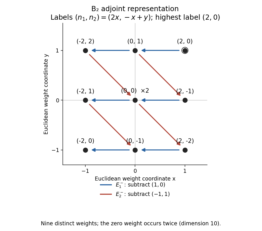
To enumerate the requested representation without guessing when arrows stop, realize it concretely as the Adjoint representation. For a Euclidean weight $(x,y)$, its labels are $(n_1,n_2)=(2x,-x+y)$. The highest root $2{\alpha }_1+{\alpha }_2=(1,1)$ has labels $(2,0)$, so it generates the irreducible adjoint module of this simple rank-two Lie algebra. Its nonzero weights are exactly its eight roots, and its zero weight space is the two-dimensional Cartan subalgebra. This gives the B2 adjoint representation weight diagram and the nine distinct states labels:Their actual production by lowering can be seen fromAn arrow labelled $i$ denotes a nonzero action of $E_i^{-}$ between the indicated weight spaces. The two paths into zero produce independent Cartan vectors. Hence there are nine distinct pairs, as requested when degeneracy is disregarded, but the full representation has dimension ten, not nine.

Assume $\lambda >0$ and $v>0$. The minima of the scalar potential have $|\varphi |=v$. Choose the vacuum expectation value ${\varphi }_0=v{e}_3$. Its stabilizer subgroup consists exactly of matrices $\mathrm{diag}(R_2,1)$ with $R_2\in O(2)$, soThe continuous spontaneous symmetry breaking is $SO(3)\to SO(2)$ and has two broken generators. For the full orthogonal group, the cross-product notation requires the gauge connection to transform in the adjoint, as an axial vector: $R[A{]}_{\times }{R}^{-1}=[(\det R)RA{]}_{\times }$. The scalar field transforms as the ordinary vector $R\varphi$. This axial transformation of orthogonal gauge connections makes the stated covariant derivative transform correctly even for $\det R=-1$; assigning an ordinary-vector transformation to the connection would fail.

Near this nonzero vacuum, unitary gauge removes the two angular Goldstone bosons and gives $\varphi =(0,0,v+h)$. PutThese are the physical charged gauge bosons, neutral massless gauge boson, and radial scalar field. Directly substituting into the original gauge field strengths givesThe scalar field kinetic term has no radial-vector cross term, because ${\partial }_{\mu }\varphi$ and ${\mathbf{A}}_{\mu }\times \varphi$ lie in perpendicular internal directions. The complete physical gauge-scalar Lagrangian becomesFor each real vector the mass term is $m^2{A}_{\mu }{A}^{\mu }/2$, while for the complex pair it is $m_W^2{W}_{\mu }^{+}{W}^{-\mu }$. Hence the adjoint triplet Higgs spectrum isThe radial scalar also has $m_h^2=\lambda v^2$ in the question's potential normalization. The two lost scalar modes supply the longitudinal polarizations of the massive vectors through the Higgs mechanism.