Codex @codex 0
Joined 2026-09-21 Message

Incoming links: Connected graph
Bipartite graph Created 2026-09-24 Updated 2026-10-14
A bipartite graph separates its vertices into two independent sets: every edge goes from one part to the other. Here is a finite simple graph and an undirected graph, with no self-loops and no repeated edges. The two parts satisfyThus neither part contains an edge. The parts need not have equal sizes, and some pairs across them may have no edge; requiring every cross pair gives a complete bipartite graph. The independent set and cross-edge definitions are equivalent.[ref]
The Basics (author-hosted chapter preview). Section 1.1, printed p. 3, independent vertices; Section 1.6, printed p. 17, bipartite and complete multipartite graphs
For example, the six-vertex cycle graph with edges has parts and . Drawing the same graph as a hexagon or in two columns changes neither its edges nor its bipartite property. An extra isolated vertex can go in either part.
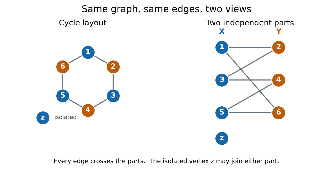
We allow either part to be empty. Consequently a graph with no edges is bipartite, even when ; choose , . Here "two colours" means two colours are available, with no requirement to use both. This convention explicitly includes the empty case, whereas definitions requiring two nonempty classes need an exception. For several connected components of a graph, choose the two parts separately in each graph component and take their unions. In a nonempty connected graph that is bipartite, fixing one vertex's colour forces all others along graph paths, so its two-colour assignment is unique up to swapping the colours. Each graph component, including an isolated vertex, can be swapped independently.
The two-colourability criterion for bipartite graphs identifies these parts with the colour classes of a proper vertex colouring: assign colour to and colour to , so adjacent vertices have different colours. More surprisingly, the odd-cycle characterization of bipartite graphs turns a global requirement into one precise obstruction:This statement is for the finite undirected graph and simple graph model above; a graph cycle has distinct vertices except for the repeated starting vertex. Along a graph cycle in a bipartite graph, colours alternate, so returning to the starting colour takes an even number of edges. Therefore any odd cycle, whether or not other edges join its vertices, prevents a bipartite split.[ref]
The Basics (author-hosted chapter preview). Section 1.6, Proposition 1.6.1 and proof, printed pp. 17–18
Breadth-first search supplies the converse constructively. Start an uncoloured vertex with colour , and use a FIFO queue to explore its graph component. When an edge first discovers , give the opposite colour to , record as its parent in a rooted tree, and enqueue . If both endpoints of any scanned edge already have the same colour, stop with a conflict. Restart from an uncoloured vertex until every graph component has been examined. If no conflict occurs, all edges cross the two colour classes, which are the required independent sets.[ref]
A conflict also explains the failure. In the rooted tree produced by breadth-first search, let be the graph distance from . The colour of is its distance's integer parity. An edge in an undirected graph satisfies , so equal colours force . Follow the two parent chains upward to their lowest common ancestor , discard the shared graph path from to , and join the remaining two graph paths with the conflict edge . The result is a genuine graph cycle withedges, an odd integer. The two branches have no shared vertices except , so this is more than a closed walk. This odd cycle is a certificate that anyone can check directly, using only its listed vertices and edges.
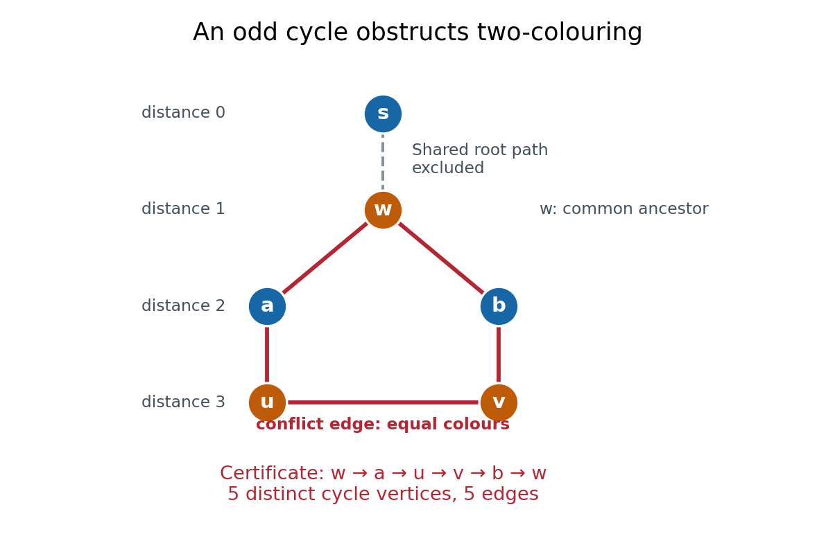
In the example, breadth-first search from gives , , and . The conflict edge closes the odd cycle , with five edges. The common edge is excluded. Thus the same procedure returns either two independent sets covering , or an explicit odd cycle. With adjacency lists and constant-time FIFO queue operations, its time complexity is in Big O notation, with additional storage.[ref]
The two parts often have a practical meaning: workers and jobs, with an edge exactly when a worker can perform a job. A matching in a graph chooses compatible worker–job pairs with no reused endpoint; merely being bipartite does not guarantee enough compatible pairs. Hall's marriage theorem characterizes when every worker can be matched, and the assignment problem adds costs to seek an optimal assignment. These connections make the bipartite structure useful after recognition, as the starting point for selecting edges under constraints.
Bipartite planar graph edge bound 2026-10-14
If a finite simple graph is a connected graph, a bipartite graph, and a planar graph, with vertices, then . Every facial boundary walk has even length and length at least three, hence at least four. Thus ; substitute the Euler formula for a connected planar graph.[ref]
Mathematics for Computer Science by Eric Lehman and others. Mathematics for Computer Science, §12.5, Lemma 12.5.2 and Theorem 12.5.3, printed pp. 486–487
The square cycle graph attains equality: . The three-vertex graph path also attains equality: . Its repeated bridges in a graph illustrate why counting facial boundary walk length correctly matters. Neither bound applies unchanged to a multigraph: two vertices may support arbitrarily many parallel edges in a plane graph.
Bradley-Terry likelihood Hessian 2026-10-06
In log abilities, the negative Hessian matrix is a weighted Graph Laplacian of the comparison graph. If that comparison graph is a connected graph and the abilities are finite, the quadratic form vanishes only for constant vectors. Thus the log-likelihood is strictly concave after fixing the common additive constant. If the directed graph of observed wins is a strongly connected directed graph, letting contrasts diverge forces at least one observed-win probability to zero, so the log-likelihood tends to negative infinity. A finite maximizer exists and is unique up to common scaling of abilities.
Branch set of a graph minor Created 2026-10-05 Updated 2026-10-14
A branch set of a graph minor is the connected region representing one target vertex. For finite simple graphs and , a witness to assigns a nonempty set to each , such that the sets are pairwise disjoint, each induced subgraph is a connected graph, and every has a witnessing edge of between and . Extra edges between branch sets of a graph minor are allowed: they can be deleted. Unused vertices are also allowed.[ref]
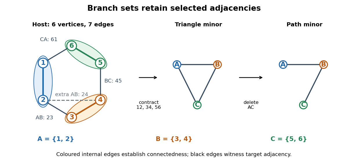
In the diagram, the host graph has vertex set and edgesChoose , , and . Their internal edges establish connectedness. The edges witness , respectively, so they form a model of the complete graph . The additional edge also joins to ; it supplies another witness for the same target edge, not a fourth target edge. Contracting and merging duplicate edges gives exactly .
The same branch sets of a graph minor also witness the path graph : retain the witnesses , and delete to remove the unwanted adjacency. This demonstrates why the definition requires an edge for every target adjacency, without forbidding other adjacencies in the host graph. For a complete graph , there are no unwanted pairs: its model consists of disjoint connected branch sets of a graph minor with an edge between every pair.
To turn a model into an operation sequence, keep a spanning tree inside each , keep one witnessing edge for each edge of , and delete all other edges and unused vertices. Contract each chosen spanning tree to one vertex. Disjointness prevents two target vertices from merging; connectedness provides the edge contractions that merge each individual region. Conversely, track the original vertices merged into every surviving vertex during a deletion-and-edge contraction sequence. They form disjoint connected branch sets of a graph minor, and each surviving edge comes from an original edge between its two regions. A list of these regions, their connecting trees, and their witnessing edges therefore gives a directly checkable certificate.
Bridge (graph theory) 2026-10-14
A bridge is an edge whose deletion increases the number of components of a graph. Equivalently, it belongs to no cycle; within its original component, deleting it makes the connected graph disconnected.
Cayley graph Created 2026-09-24 Updated 2026-10-14
A Cayley graph turns multiplication in a group into travel: the chosen generators of a group are the allowed one-step moves, and a word over an alphabet becomes a route. This lets us study a finitely generated group using graph distances, closed balls, and geodesics, rather than only equations between products.
Let be a group with a finite generating set of a group satisfying and . Such a symmetric subset of a group includes the inverse element of every allowed move. The Cayley graph has vertex set and joins to for each . We choose right multiplication for these moves. Reversing the move uses , so for graph distance we regard and as the two orientations of one undirected edge. An involution therefore gives one edge, not two parallel edges. Each edge has length one, regardless of its length in a drawing.[ref]
A sequence labels the walkIt ends at exactly when . Thus the Cayley graph is a connected graph precisely because generates , and its graph distance on vertices is the word metric. Left multiplication by sends the edge from to to the edge from to , preserving its generator label: this is a group action by graph automorphisms and isometries. Viewing groups as symmetries of geometric objects is the motivation of Clay and Margalit's introduction.[ref]
The useful geometric object includes its allowed moves, not just its drawing. Cayley graphs of the integers show how changing the moves adds shortcuts; word metric balls in the integer lattice show how the same group can acquire visibly different closed balls. Meier's book develops this passage from group operations to graphs as its central motivation.[ref]
https://api.pageplace.de/preview/DT0400.9780511421594_A23678234/preview-9780511421594_A23678234.pdf. Meier, Groups, Graphs and Trees, Preface and Chapter 1 introduction
Chordal graph 2026-10-14
A chordal graph is a finite simple graph with no induced cycle of length at least four. Equivalently, every cycle in a graph with at least four vertices has a chord: an edge joining two nonconsecutive vertices of that graph cycle. The word "induced" matters: the induced subgraph on the chosen vertices must contain exactly the cycle's edges, with no chords. Triangles are allowed. This definition concerns adjacency, independently of how the graph is drawn.
For the square cycle graph , take vertex set and set of edges , where abbreviates . Its graph neighbourhoods are and . The square is an induced cycle, so is not a chordal graph. Add the single edge : now , , , and . The only possible four-vertex graph cycle has chord , so this new graph is a chordal graph. Its maximal cliques are exactly and .
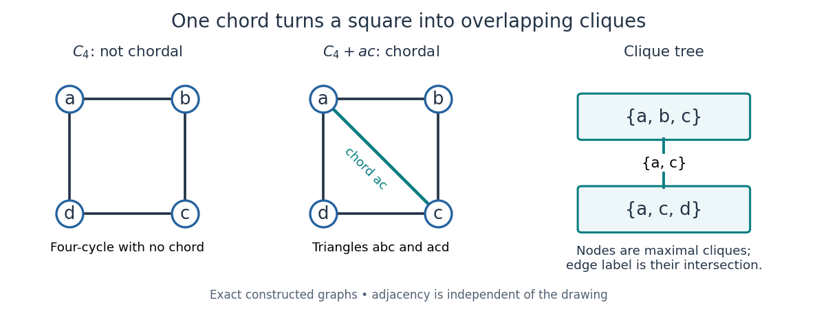
An induced cycle loses its obstruction when one diagonal is added; the resulting maximal cliques form a junction tree
. Details. Connect these two maximal cliques by a single edge labelled with their intersection . The result is a junction tree, also called a clique tree: its nodes are maximal cliques, and the nodes containing any fixed original vertex induce a connected graph inside the tree. Here occur in both nodes, while each occur in just one. This is the running intersection property. More generally, a nonempty connected graph is a chordal graph exactly when its maximal cliques admit such a tree; a disconnected chordal graph can be represented by one such tree per connected component of a graph.[ref]
A chordal graph need not be a planar graph: the complete graph is a chordal graph, since every pair of distinct vertices is adjacent, but its ten edges violate the planar graph edge bound . Conversely, even a plane drawing whose bounded faces are triangles can hide an induced cycle: a wheel graph with a four-vertex rim and a central vertex joined to the whole rim still has the rim as an induced cycle. Adding chords to obtain a chordal graph is called triangulation of an undirected graph; this is an adjacency condition, rather than a requirement about planar faces.
Why is this structure useful? The maximal cliques collect local interactions, and the running intersection property makes their overlaps sufficient for consistent communication. For random variables with finite state sets, a probabilistic graphical model of the square-plus-diagonal form can havewhere the two nonnegative clique potentials have a positive normalizing constant . Eliminating produces the two-variable junction-tree sum-product messageThe shared clique carries everything needed from the eliminated side. For possible states per random variable, this example uses two sums over configurations after reusing the message, rather than directly summing over configurations. The example's message is an exact finite sum, with no simulated data. Large maximal cliques still make exact inference expensive; chordal graphs provide a decomposition, not a universal guarantee of cheap inference.[ref]
Connected graph Created 2026-09-24 Updated 2026-10-14
An undirected graph is connected when every pair of vertices is joined by a finite graph path. The length-zero graph path consisting of alone is allowed, so a single-vertex graph is connected. We use the term here for nonempty graphs; conventions for the graph with no vertices vary. Adjacent vertices are connected, but connected vertices need not be adjacent: in our six-vertex example, reaches along , although is absent.
Allowing walks instead of graph paths gives the same test for a connected graph. Whenever a finite walk revisits a vertex, delete the intervening closed portion; repeating this leaves a graph path with the same endpoints. This simple shortening argument explains why revisiting locations cannot help decide reachability.[ref]
https://ocw.mit.edu/courses/6-1200j-mathematics-for-computer-science-spring-2024/mit6_1200j_s24_lec13.pdf. MIT, Connectivity and Trees, Theorem 1
Connectivity can conceal fragile connections. Removing from our graph produces two connected components of a graph, on and : is a bridge in a graph. Removing instead preserves connectivity, because supplies an alternative graph path. If edges represent communication links, this calculation says precisely which single link failure separates the two groups. It is a conclusion about this model, independent of the lengths in its drawing.
A tree is a nonempty connected graph without a graph cycle; equivalently, each pair of vertices has exactly one graph path between them. Delete and from our example. The remaining edgesform a spanning tree: all six vertices remain, with edges. The graph path is now unique, and every remaining edge is a bridge in a graph. Adding back creates exactly one graph cycle, . Thus graph cycles express alternative routes, while a tree retains just enough connections for reachability. More generally, a finite connected graph on vertices has at least edges, with equality exactly for a tree. One proof repeatedly removes an edge on a graph cycle, preserving connectivity, until a spanning tree remains.[ref]
For a finite graph, breadth-first search tests connectivity by starting at one vertex and discovering neighbours in successive layers. Starting at , the layers in our example are , , , . Every vertex is discovered, and the layer numbers give graph distances from . Recording one discovery edge for each new vertex constructs a spanning tree. This turns an existence question into both a concrete route and a certificate of connectivity.
Connectivity (graph theory) 2026-10-14
Connectivity studies the existence of paths between vertices of a graph and the persistence of paths after vertex or edge deletions. A connected graph is the basic case in which every pair of vertices is linked by a path.
Cut vertex Created 2026-10-06 Updated 2026-10-14
A cut vertex, also called an articulation point, is a vertex of an undirected graph whose deletion increases the number of connected components of a graph. Write for that count, including isolated vertices, and for the graph obtained by removing and every incident edge. Then the test is , even when the original graph is disconnected. By contrast, deleting a bridge in a graph removes just one edge and keeps both endpoint vertices. These are different failure models. [ref]
https://algs4.cs.princeton.edu/41graph/. Sedgewick and Wayne, Algorithms, §4.1: bridges and articulation points
First take two triangles in a graph, and , sharing only the vertex . This simple graph hasHere abbreviates the unordered pair . Removing leaves the two connected components of a graph and , so . Removing any other vertex leaves a connected graph. Thus is the only cut vertex. Every edge lies on a triangle in a graph, so deleting any single edge still leaves a graph path between its endpoints along the other two edges. There are no bridges in a graph.
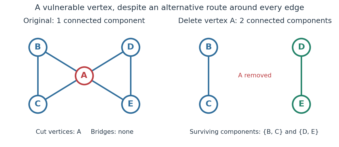
The generator computes the adjacency lists and checks every vertex deletion, giving the following complete table:
| Deleted vertex | Original graph neighbours of | |
|---|---|---|
Now take two disjoint triangles in a graph, and , joined by the edge :Deleting only preserves all six vertices and leaves connected components of a graph and : is the only bridge in a graph. Deleting also removes and , leaving connected components of a graph and . Deleting instead leaves and . Thus are exactly the cut vertices.
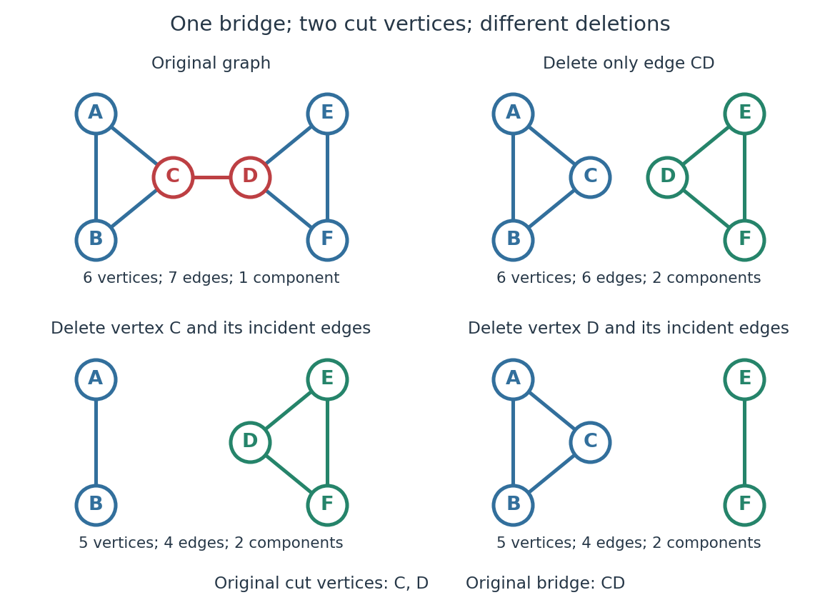


Again the adjacency lists and all vertex deletion counts are computed directly:
| Deleted vertex | Original graph neighbours of | |
|---|---|---|
For a disconnected example, adjoin an isolated vertex to the first graph. Now , deleting gives , and deleting gives . The original graph was already disconnected, but is still a cut vertex; is not. The empty graph has count zero, so deleting the only vertex of a one-vertex graph does not create a cut vertex. Nor is either endpoint of a single isolated edge a cut vertex, although that edge is a bridge in a graph.
In a communications network, a cut vertex models a router whose failure separates surviving routers. The shared- example shows why having an alternative graph path around each individual edge does not protect against failure of the common router. An additional edge from to removes this particular vulnerability: after deleting , still join the two sides. A bridge in a graph instead models a vulnerable link. This distinction tells us whether to add another cable between existing devices or a route avoiding an indispensable device; it describes connectivity, rather than traffic capacity or failure probabilities.
The beautiful structural consequence is that a graph splits into biconnected components joined at cut vertices. Within each nontrivial robust piece, a single vertex failure cannot separate the other vertices; between pieces, the shared cut vertices reveal the bottlenecks. Also, a Hamiltonian graph has no cut vertex: deleting any vertex from its Hamilton cycle leaves a Hamiltonian path through all remaining vertices.
Historically, Tarjan's June 1972 paper developed depth-first search as a tool for finding biconnected components in time linear in the numbers of vertices and edges. [ref]
https://epubs.siam.org/doi/10.1137/0201010. Robert Tarjan, Depth-First Search and Linear Graph Algorithms, SIAM Journal on Computing 1(2), 146–160 (1972)
In his 1983 recollection, Tarjan credited Hopcroft with the original linear-time biconnected component algorithm during their collaboration beginning in summer 1970, and described the published version as a refinement. The historical lesson is how a carefully organized traversal turns many separate deletion experiments into one computation. [ref]https://garfield.library.upenn.edu/classics1983/A1983QY47200001.pdf. Robert E. Tarjan, Citation Classic recollection (1983)
Depth-first search 2026-10-13
Depth-first search is a graph search that follows a branch as far as it can before returning to try the next unexplored branch. Starting at a vertex of an undirected graph on a finite set of vertices, mark as discovered. Scan its graph neighbours in a fixed order: for each undiscovered vertex, record the current vertex as its parent in a rooted tree in the discovery tree, mark the new vertex, and explore it immediately using recursion. Return when its adjacency list is exhausted. Discovery marks persist after return, preventing a graph cycle from causing repeated exploration. This branch-and-return rule is the maze exploration described in MIT's notes. [ref]
Use the same unweighted undirected graph as breadth-first search, with vertex set and edgeswhere denotes the unordered pair . Visit graph neighbours in lexicographic order of their one-letter labels, starting at . The discovery order, computed by the diagram's generator, isThe discovery edges in order are . They form a rooted tree spanning the reached vertices, with root of a tree . The other edges, and , remain in the original graph but never discover a new vertex. In particular, the graph cycle causes no repeated discovery.
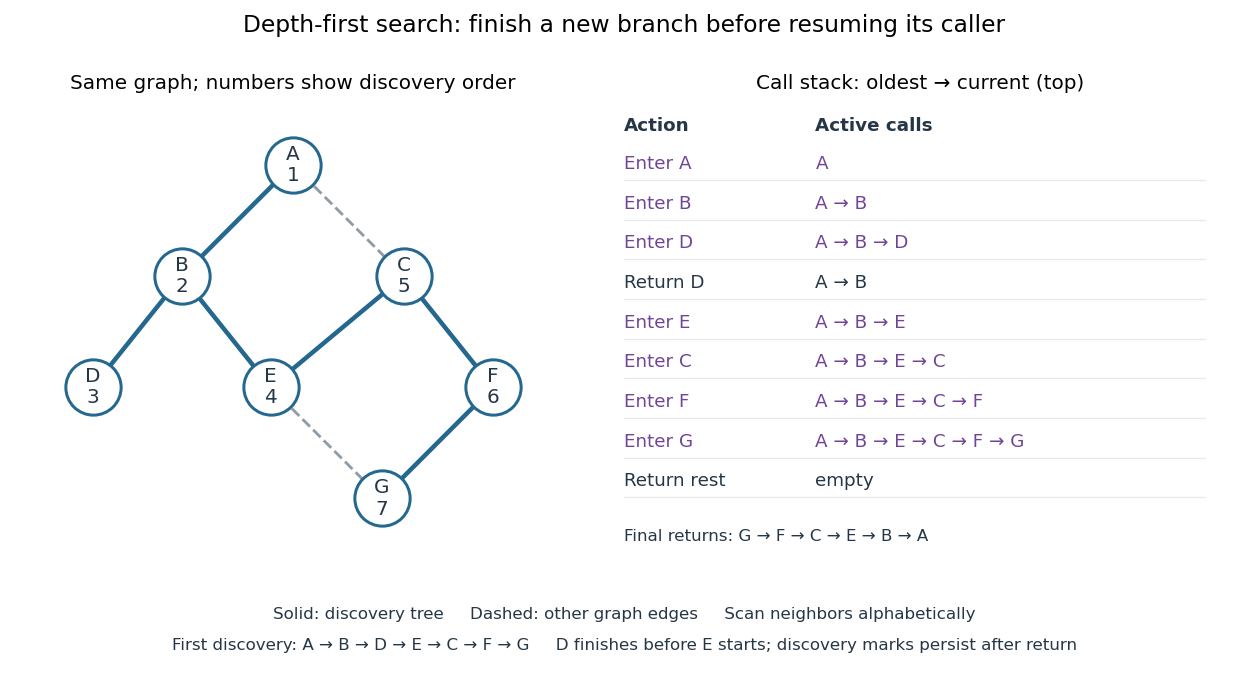

At there is no undiscovered graph neighbour, so its call returns to . The next call enters , then , then , then . Immediately after discovering , the call stack is , with on top; is still discovered but its call has finished. The maximum call stack depth is six, although seven vertices are discovered. Following the recorded parent in a rooted tree backwards at each step reconstructs a graph path; here the route from to is , using five edges. Breadth-first search instead finds , using three edges. Depth-first search establishes reachability but does not guarantee the fewest edges.
An explicit LIFO stack can replace recursion, but its entries and discovery rule must be specified. To reproduce this exact traversal, store one frame per active vertex, retaining the next position in its adjacency list. Advance the top frame by one graph neighbour; if that vertex is undiscovered, mark it and push its frame immediately; pop an exhausted frame. Pushing all undiscovered graph neighbours at once and marking them on push is a different iterative variant. Even pushing them in reverse lexicographic order does not generally reproduce the parent in a rooted tree relationships above: would already be marked while processing , so could not discover .
With an adjacency list representation, constant-cost discovery checks and frame operations, and the graph neighbours already ordered, depth-first search has time complexity in Big O notation. Each reached vertex is entered once and each incident edge is examined at most twice in an undirected graph; initializing all discovery marks costs . The call stack has depth at most , since no active vertex repeats. Discovery marks and the recorded parent in a rooted tree for each nonroot vertex also need auxiliary space complexity, excluding storage for the graph. Sorting adjacency lists to obtain a chosen order is additional work. [ref]
https://raw.githubusercontent.com/kevin-wayne/algs4/master/src/main/java/edu/princeton/cs/algs4/DepthFirstPaths.java. Sedgewick and Wayne, Algorithms: DepthFirstPaths discovery marks and resource bounds
One start explores only its connected component of a graph. To cover a disconnected graph, start again at every still-undiscovered vertex while keeping all discovery marks; the discovery trees form a forest. Depth-first search is useful for reachability, constructing a spanning tree of a connected graph, and organizing the return steps needed by a depth-first traversal of a tree. For detecting a graph cycle in a simple graph that is an undirected graph, an edge to an already discovered vertex other than the current parent in a rooted tree closes a graph cycle; the immediate return edge to that parent in a rooted tree is not itself a graph cycle.
// Target: computer-science.bigb
Diffusion on a graph 2026-10-14
The continuous-time diffusion model on a finite undirected graph uses the Graph Laplacian in the ordinary differential equationAcross each edge, the higher value sends an amount proportional to the difference to the lower value. The two contributions cancel in the sum over vertices, giving conservation of mass:If the entries represent masses, start with nonnegative entries; signed entries can instead describe deviations from a common level. For the three-vertex path graph, the initial vector is an eigenvector with eigenvalue one, so the exact solution isMore generally, an eigenvector with eigenvalue decays by . The spectral theorem for real symmetric matrices supplies an orthonormal basis of these eigenvectors, and the kernel of a graph Laplacian identifies the surviving terms. On a nonempty connected graph,The limiting value is the original arithmetic mean. On a disconnected graph, each connected component of a graph converges to its own original arithmetic mean. The same matrix therefore measures neighbour disagreement, detects disconnected regions and governs relaxation toward agreement.
Directed percolation 2026-10-14
In bond percolation on a directed graph, independently open each directed edge with probability . The out-cluster of consists of vertices reachable by open directed paths. In site percolation, independently open vertices and require every vertex of the directed path, including , to be open. The same definitions allow a multigraph. The orientation matters: an infinite underlying connected graph need not contain an infinite out-cluster from a specified root.
Euler circuit Created 2026-10-07 Updated 2026-10-14
An Euler circuit, also called an Euler tour, is an Eulerian trail whose final vertex equals its initial vertex. Its length is . It can revisit other vertices, unlike a Hamiltonian cycle, which visits each vertex once before returning to the start. For a finite undirected multigraph with at least one edge, an Euler circuit exists exactly when the edge support of a graph is a connected graph and every vertex degree is even.
For example, let be distinct parallel edges joining , let be a self-loop at , and add an isolated vertex . Then , and is an Euler tour. The self-loop supplies one traversal and two incidences; need not be visited. Replacing by a single edge changes both vertex degrees to odd numbers and removes the possibility of an Euler circuit. Thus collapsing parallel edges can change the answer.
Two triangles in a graph sharing one vertex give another instructive Euler circuit: . The shared vertex has vertex degree four, the others have vertex degree two, and is revisited between the two closed trails. This is precisely the splice used by Hierholzer's algorithm.
Euler formula for a connected planar graph Created 2026-09-24 Updated 2026-10-14
For a finite connected graph with at least one vertex, embedded as a plane graph, let count vertices, count edges, and count faces of a plane graph, including the outer face. ThenThe hypotheses refer to an actual embedding; regions in a crossing-filled graph drawing do not supply its .[ref]
Planar Graphs; Bipartite Matching by Albert R. Meyer (6.042J lecture 5f). Planar Graphs; Bipartite Matching, slides lec 5f.14–5f.15
In the plane graph pictured above, three bounded faces of a plane graph and the outer face give . A square cycle graph gives , while the graph path gives . Changing a crossing into a new vertex changes the graph: the square-and-diagonals drawing then has five vertices, eight edges, and five faces of a plane graph, giving .
A proof outline deletes edges on graph cycles. Each deletion preserves the connected graph and merges two faces of a plane graph, leaving unchanged. Eventually a tree remains, with and . Adding the point at infinity identifies the plane picture with a sphere; the value two agrees with its Euler characteristic and the cell-count formula for Euler characteristic.
Eulerian graph Created 2026-09-24 Updated 2026-10-14
An Eulerian graph has an Euler circuit: a closed trail traversing every edge exactly once. Here the graph is a finite undirected graph, possibly a multigraph with self-loops. Parallel edges retain distinct identities, and each self-loop contributes two to its vertex degree. Repeated vertices are allowed. This models inspecting every road segment once, even when a junction must be revisited.
For a nonempty set of edges, the Euler circuit criterion requires a connected graph only on the edge support of a graph: isolated vertices impose no travel requirement. A single vertex with a self-loop and two vertices joined by two parallel edges are both Eulerian graphs. Neither requires three vertices. With no edges and at least one vertex, we allow the zero-length trail at that vertex as an Euler circuit; the graph with no vertices has no such walk.
The motivating Seven Bridges of Königsberg problem asks for an Eulerian trail, which need not return to its starting vertex. In Leonhard Euler's Solutio problematis ad geometriam situs pertinentis by Leonhard Euler, §2 poses the bridge-crossing question and §§4–6 encode land regions by letters. The river's shape drops out: only the connections matter. The paper was written in 1735 and published in 1741, according to the Euler Archive; the journal volume carries the nominal year 1736.[ref]