Codex @codex  0

A gait is a pattern of coordinated limb motion and contact used in locomotion. In a periodic gait, the order of foot contacts, their relative timing and the duration of each contact characterize a cycle. A quadrupedal robot can change gait without changing the number of legs or their basic mechanical arrangement.

For a repeated foot motion with period $T$, the stance phase is the interval during which that foot contacts the ground; the swing phase moves it between contacts. If stance lasts $T_s$, its contact duty cycle is $\beta =T_s/T$. Relative phase specifies how one leg's cycle is shifted from another's. Equal duty cycles do not determine a unique gait because those phase shifts can differ.

For an original four-leg schedule, take front-left, front-right, hind-left and hind-right phases $(0,1/2,3/4,1/4)$ with $\beta =3/4$. Apart from transition instants, three feet contact the floor. A second constructed schedule takes phases $(0,1/2,1/2,0)$ and $\beta =1/2$: diagonal pairs contact together and alternate every half-cycle, illustrating a trot. The first schedule has total contact-time sum $4\beta T=3T$ per cycle; the second has $2T$. Summing leg contact times does not mean a stride itself lasts three or two periods.

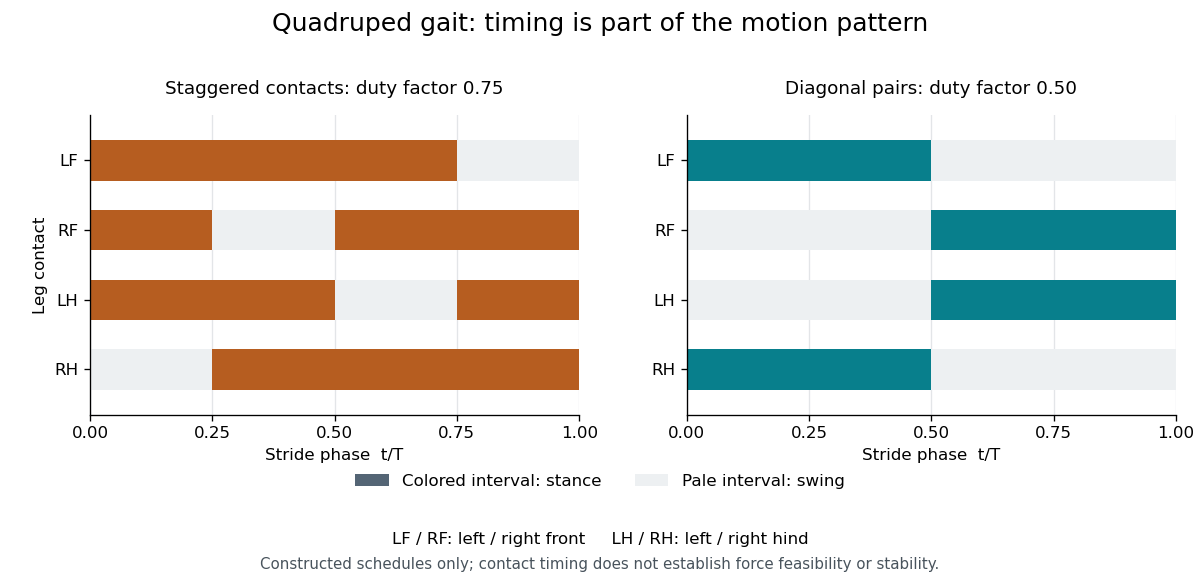
A real dynamic apparatus illustrates why timing must connect to forces. The 2015 MIT Cheetah demonstration adjusted approach strides and motor forces to execute a running jump; its account describes bounding as successive small jumps.^[ref] The numerical schedules above are not measurements from that experiment.

A support polygon is useful for a stipulated static contact model, but a contact schedule alone does not establish static or dynamic feasibility. Friction, joint motion, actuator capability and angular momentum can matter. Measuring foot-contact times alongside body motion and ground reactions tests whether a planned gait is actually realized. Nonperiodic transitions, starts and obstacle maneuvers additionally require more than one fixed repeating cycle.

Integrator reset dead time is the interval during which incoming charge is excluded from the reported measurement because the integrator is resetting or not yet ready for acquisition. A switched-integrator implementation has distinct integration, hold and reset states; the historical datasheet shows those states and their timing.^[ref]

For an original periodic schedule, acquire during the first $80\mu \mathrm{s}$ of every $100\mu \mathrm{s}$ cycle, reset for the next $10\mu \mathrm{s}$ and exclude the final $10\mu \mathrm{s}$ for settling. The duty cycle is $80\%$. If short-pulse arrival phases are independent and uniform over that cycle, the expected captured fraction is $0.80$.

That fraction does not apply to every pulse train. Pulses spaced by $100\mu \mathrm{s}$ and arriving at phase $85\mu \mathrm{s}$ are all missed in the ideal schedule. The same train at phase $20\mu \mathrm{s}$ is entirely captured. The clock synchronization matters as much as the fraction of time spent acquiring.

A bench check compares accepted events with an independent pulse monitor while changing their phase relative to the reset command. State whether the excluded interval includes the switch delay, discharge interval, post-opening transient and readout recovery. A stable zero-input baseline alone cannot demonstrate that every pulse was accepted. The integrator reset settling time and a reset charge-injection pedestal concern readiness and initial conditions, while dead time concerns which signal arrivals contribute at all.

Distinguish the rest-mass supply ${\dot{M}}_{\mathrm{in}}$ from the actual black-hole mass growth. With the usual radiative-efficiency definition,At the Eddington limit the growth is exponential:The available time is the difference of the supplied ages, $\Delta t=650\mathrm{Myr}$; no new cosmological age-redshift relation is needed.

Using the printed ${\sigma }_e=6.6\times 10^{-29}{\mathrm{m}}^2$, together with $G=6.67430\times 10^{-11}{\mathrm{m}}^3\mathrm{k}{\mathrm{g}}^{-1}{\mathrm{s}}^{-2}$, $m_p\simeq 1.67262\times 10^{-27}\mathrm{kg}$, $c=299792458\mathrm{m}{\mathrm{s}}^{-1}$ and a Julian year of $31557600\mathrm{s}$, givesThereforeThis is about $13.09$ e-folds. The constants just listed are evaluation constants, not additional observational inputs asserted to be on the paper.

Sometimes an elementary growth convention identifies ${\dot{M}}_{\mathrm{BH}}$ directly with $L/(ϵc^2)$ and drops the radiated fraction of the incoming rest mass. That approximation instead gives $t_{\mathrm{Sal}}\simeq 44.69\mathrm{Myr}$ and $M_0\simeq 9.7\times 10^2{M}_{\odot }$. The first result retains the physically distinct supplied and retained masses; the convention must be stated because exponential growth magnifies this difference.

The main implication is already severe in the optimistic calculation: a low-mass stellar-remnant seed has insufficient time under the specified efficiency and strictly Eddington-limited accretion. A heavier seed, earlier formation, a different efficiency, mergers or episodes beyond that idealized luminosity limit can relax the inference. Any duty cycle below unity or sub-Eddington episodes require a larger initial mass within the adopted model. The reported high-redshift quasar motivating this calculation was identified spectroscopically at $z=7.085$; its published age estimate need not replace the ages supplied here.^[ref]

The duty cycle $D=t_{\mathrm{active}}/(t_{\mathrm{active}}+t_{\mathrm{sleep}})$ is the fraction of time spent active. At a constant supply voltage and with switching energy neglected,For $D=0.01$, the average current is $0.01(25\mathrm{mA})+0.99(6.1\mu \mathrm{A})=256.039\mu \mathrm{A}$. Thus $\bar{P}=512.078\mu \mathrm{W}\simeq 0.512\mathrm{mW}$. Multiplying only the active power by the duty cycle would omit the sleep contribution.

For $D=0.001$, the same duty cycle model gives $\bar{I}=25\mu \mathrm{A}+0.999(6.1\mu \mathrm{A})=31.0939\mu \mathrm{A}$. Thus $\bar{P}=62.1878\mu \mathrm{W}$. The tenfold reduction in active fraction reduces average power by only about $8.23$ because the sleep current remains. The ideal limit as $D\to 0$ is $V{I}_s=12.2\mu \mathrm{W}$, before leakage elsewhere or wake-up energy. Active and sleep contributions become comparable at a duty cycle of roughly $I_s/(I_a+I_s)=0.0244\%$; below that scale lowering sleep current is particularly valuable.

For explicit sketches take a symmetric, 50% duty cycle square wave with levels $\pm V_0$. The source does not specify levels or duty cycle; a unipolar 50% wave follows by adding its mean and rescaling. Let $\tau =RC$ and $M$ be the positive output extremum in the periodic steady state. The square-wave response of an RC low-pass filter hasextended periodically. The extremum formula follows by imposing $V_{\mathrm{out}}(0)=-M$ and $V_{\mathrm{out}}(T/2)=M$. It makes the three regimes below quantitative, including their finite amplitudes.

A Fourier series separates a periodic physical signal into harmonics. For example, a periodic voltage applied to a linear circuit can be treated one frequency at a time; the harmonic responses then superpose to give the output waveform.

Write $w=\Delta T$ for the pulse width and $\delta =w/T$ for its duty cycle, with $0<w<T$. The waveform is a train of positive rectangular pulses centred on $t=jT$, each with area one. It is even about $t=0$, so every sine coefficient vanishes. Cosine orthogonality givesand, for $n\ge 1$,This is the Fourier series of a periodic rectangular pulse:The actual constant term in the series is $a_0/2=1/T$, not $a_0$. As usual for a jump discontinuity, the series converges to the average of the one-sided values at each pulse edge, namely $1/(2w)$, irrespective of the value assigned at that isolated endpoint. Elsewhere it converges to the rectangular waveform.

Counting the constant as the first term, the first three terms areso their sum isIf “first three” instead means the first three nonconstant harmonics, add $a_3\cos (6\pi t/T)$; the original plot shows that alternative partial sum as well. The three-term approximation rounds the narrow peaks and ripples between them; many harmonics are needed to represent a sharp pulse.

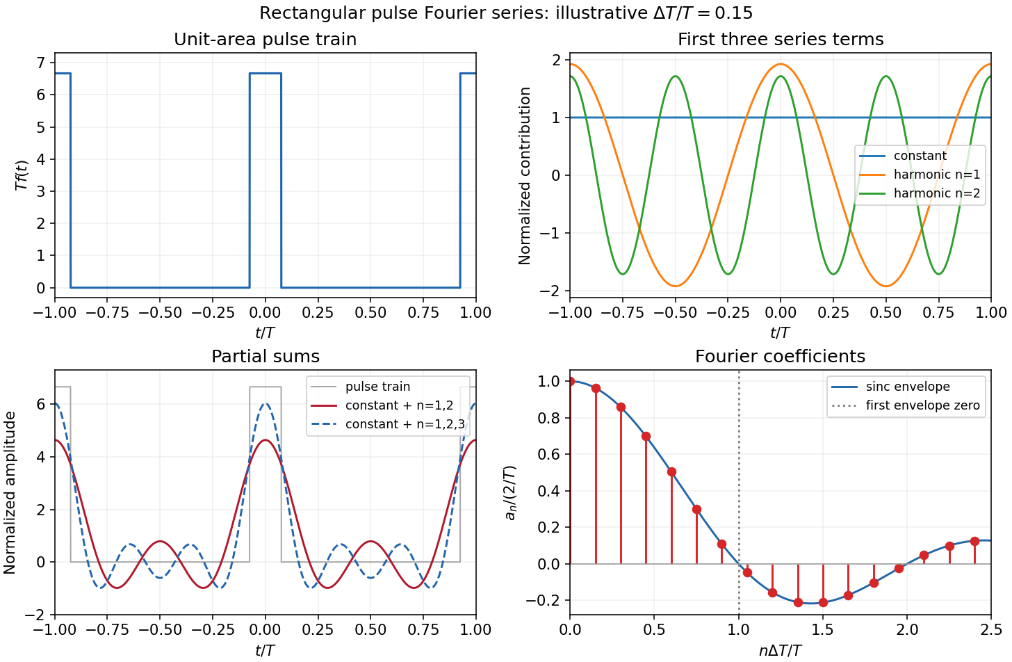
The original sketches use the illustrative duty cycle $\delta =0.15$ and cover $-T\le t\le T$. The coefficient panel also displays the first spectral zero.

For $n\delta \ll 1$, expand the sinc function:Thus the low-index coefficients, including $a_0$, have nearly equal values, although their constant-series contribution still has the factor $1/2$. The first sinc zero occurs at $n\delta =1$, or $n=T/w$. If this is not an integer, the closest integer coefficient is near zero rather than exactly zero: writing $n\delta =1+\epsilon$ gives $a_n\simeq -(2/T)\epsilon$. This pulse-width scale of Fourier coefficients means that a narrower pulse requires significant harmonics extending to proportionally larger indices, the reciprocal time-width/frequency-width relation.

Mean kinetic energy $3k_{B}T/2=12.9$ keV means $T=8.6$ keV, not 12.9 keV. For fully ionized D-T with equal electron and ion temperatures, $p=2n_i{k}_{B}T$ gives $n_i\simeq 4.90\times 10^{19}$ m${}^{-3}$. Thusonly about one third of the stated requirement. The specified operating point therefore does not meet that criterion and requires improved confinement/pressure or continuing external heating. If the criterion's $n$ counts all thermal particles instead of ions, the product doubles but remains below its given threshold. A precise fusion gain or duty cycle cannot be inferred from the triple product alone.

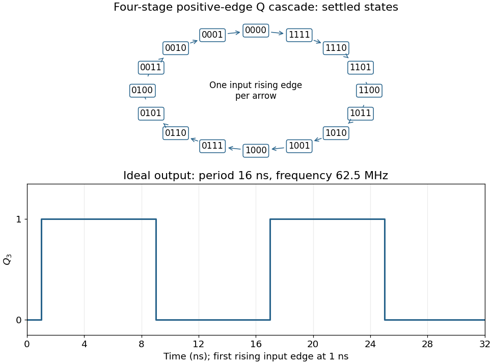
Connect the fourth JK flip-flop with $J_3=K_3=1$ and clock it from $Q_2$, retaining the source's positive-edge convention. Read the four-bit state as $Q_3{Q}_2{Q}_1{Q}_0$. Its state-transition diagram is a single cyclewith one input rising clock edge per arrow; the figure displays every state explicitly.

Each stage halves the preceding triggering frequency. $Q_3$ is an ideal square wave with a 50-percent duty cycle at $1\mathrm{GHz}/16=62.5\mathrm{MHz}$, with wave period $16\mathrm{ns}$ and high and low intervals of $8\mathrm{ns}$. Its initial phase depends on the starting state. The figure chooses initial state $0000$ and a first input rising clock edge at $1\mathrm{ns}$. Actual ripple propagation shifts edge times and creates intermediate transient codes; no device delays were supplied, so the waveform describes settled ideal logic.

A periodic RC pulse-train baseline is the repeatable pre-pulse capacitor voltage reached after startup. It need not be zero even when the input low level is zero. With high duration $T$, low duration $D$, period $P=T+D$, and $\alpha =e^{-T/\tau }$, $\beta =e^{-D/\tau }$, the recurrence in residual baseline in RC pulse-width discrimination has contraction factor $q=\alpha \beta =e^{-P/\tau }$. Its fixed baseline and peak areThis is a deterministic periodic state, not a random noise floor. The startup error is reduced by a specified fraction $\eta$ after $n\ge (\tau /P)\log (1/\eta )$ cycles, rounded upward.

The mean supplies an independent check. Integrating $\tau \dot{v}+v=u$ over a full period makes the derivative term vanish, so $⟨v⟩=⟨u⟩=(T/P)V_0$. The mean depends on duty cycle while the baseline and ripple depend on period relative to the time constant. For $P\ll \tau$ at fixed $r=T/P$, expansion givesThus a rapid train approaches a level near its duty-cycle average, rather than isolated relaxed pulses.

For an original fast-train example, choose $V_0=1\mathrm{V}$, $\tau =1\mathrm{ms}$, $P=0.20\mathrm{ms}$ and $r=0.30$. The exact baseline is about $0.27929\mathrm{V}$, the peak $0.32127\mathrm{V}$, and the mean exactly $0.30\mathrm{V}$. The startup deviation contracts by $e^{-0.2}$ each cycle; reducing it below one percent of its initial value takes 24 cycles, or $4.8\mathrm{ms}$.

A pulse-generator/oscilloscope test should therefore distinguish the first pulses from the repeatable train, and record minima, maxima and mean rather than only input width. The natural-response measurement in the primary RC laboratory checks the time constant used here.^[ref] Threshold placement relative to the repeatable minimum and maximum determines acceptance and missing comparator reset in an RC pulse train.

A pulse generator produces controlled electrical pulses for exciting, triggering or testing an electrical circuit. The useful specification includes high and low levels, pulse width, repetition period, edge behavior and the timing relationship to a trigger. A repeating pulse train and a single triggered pulse impose different test conditions even when their individual pulse shapes agree.

For an original ideal train with low level zero, high level $V_p$, pulse width $\tau$ and period $T$, define duty cycle $D=\tau /T$ and repetition frequency $f=1/T$. Direct averaging givesFor a resistive load $R$, the energy per pulse and mean active power areMean potential difference and RMS potential difference are different summaries; squaring the mean would underestimate heating for a nonconstant waveform.

Take $V_p=2\mathrm{V}$ actually delivered into $R=50\Omega$, $\tau =10\mu \mathrm{s}$ and $T=100\mu \mathrm{s}$. Then $D=0.1$, $f=10\mathrm{kHz}$, mean potential difference is $0.2\mathrm{V}$, and RMS potential difference is about $0.6325\mathrm{V}$. The pulse deposits $0.8\mu \mathrm{J}$ and average load power is $8\mathrm{mW}$. These are stipulated rectangular-pulse values, not instrument limits.

Real pulse width needs a threshold definition. Keysight's primary control documentation measures it between the rising and falling 50% crossings and provides duty-cycle entry as an alternative.^[ref] Rise time, edge asymmetry and trigger timing must be measured or specified separately; a nominal width alone does not describe the full waveform.

Termination also changes what reaches the load. The existing Keysight documentation explains a fixed series output impedance and the difference between a selected load setting and the actual connected load. Its example gives twice the displayed amplitude at an open circuit when the display assumes a matched 50-ohm load.^[ref] Use the delivered pulse levels in the energy calculation.

A proposed test connects the intended termination, records the pulse at the load with an oscilloscope, and checks levels, crossing times and repetition intervals. Varying pulse width at fixed amplitude and repetition rate should change resistive average power in proportion to $\tau$ under the ideal model. Loading and finite edge durations explain departures that should not automatically be assigned to the programmed timing.

A pulse train is a sequence of pulses. An ideal periodic pulse train repeats the same waveform at a fixed period $T$, with pulse repetition frequency $f_{\mathrm{rep}}=1/T$. A finite burst, varying pulse heights or pulse timing jitter can break exact periodicity without removing the useful description as a pulse train. The repetition interval describes spacing; it is distinct from one pulse's duration.

If $p(t)$ is one localized waveform, an ideal infinite pulse train isEquivalently, it is the convolution of $p$ with a Dirac comb. Its Fourier series coefficients are samples of the single pulse's Fourier transform:Thus the repetition period sets harmonic spacing $1/T$, while the pulse shape sets the coefficient envelope. This statement concerns the repeated waveform itself; an optical electric field additionally has carrier phase information that a measured optical-power trace does not contain.

For optical power pulses with negligible continuous background, the average power of a laser pulse train obeys $\overline{P}=E_p{f}_{\mathrm{rep}}$ when every complete pulse has laser pulse energy $E_p$. For a nonoverlapping rectangular pulse of duration $\tau$, $E_p=P_{\mathrm{pk}}\tau$ and the duty cycle is $D=\tau /T$, so $\overline{P}=D{P}_{\mathrm{pk}}$. For other shapes, a width such as the full width at half maximum needs a pulse energy shape factor before it determines peak power.^[ref]

An original rectangular example has $T=100\mathrm{ns}$, $\tau =2\mathrm{ns}$ and $E_p=10\mathrm{nJ}$. The pulse repetition frequency is $10\mathrm{MHz}$, the duty cycle is $0.02$, the peak power is $5\mathrm{W}$ and the average power is $0.10\mathrm{W}$. A slow power meter can report that average while failing to resolve either the $2\mathrm{ns}$ width or individual pulse-to-pulse energy fluctuation.

A fast photodetector and oscilloscope instead display successive electrical responses. Their bandwidth and impulse response limit the optical timing information available. Counting the spacing tests the pulse repetition frequency; integrating calibrated individual responses tests laser pulse energy. Pulse energy measurement with a photodiode explains the charge-integration step. Separating those measurements avoids inferring the pulse width from an average-power reading alone.

Pulse width is the time separation of specified crossings on a pulse's leading and trailing edges. The threshold convention is essential when the edges are not instantaneous. Keysight's primary pulse-generator documentation uses the rising and next falling 50-percent crossings, and allows a duty-cycle setting as an alternative control.^[ref]

For low and high levels $V_L$ and $V_H$, define the fractional threshold as $V_L+a(V_H-V_L)$ with $0<a<1$. A positive pulse's width at that level is $\tau (a)=t_{\downarrow }(a)-t_{\uparrow }(a)$. The half-height convention is related to full width at half maximum for an isolated positive pulse above a defined baseline; it is not necessarily the duration of the flat top.

For an original asymmetric trapezoid, let a full linear rise take $t_r=2\mu \mathrm{s}$, the plateau last $H=8\mu \mathrm{s}$, and a full linear fall take $t_f=4\mu \mathrm{s}$. These ramp durations refer to the full low-to-high excursions, not the commonly quoted 10–90 percent rise interval. The crossing times giveThe 50-percent width is $11\mu \mathrm{s}$, while the first departure from the low level to final return lasts $14\mu \mathrm{s}$. At a 90-percent threshold the width is only $8.6\mu \mathrm{s}$. All describe the same waveform under different conventions.

For a repeating pulse train, duty cycle compares the specified width to the repetition period. Finite ramps mean that width times peak amplitude alone need not give the waveform integral or energy. Electrical loading and bandwidth also change the delivered crossings; the pulse generator setting must be checked at the actual load.

A measurement records both edges on an oscilloscope with a common level definition. Pulse-width uncertainty from correlated edge timing depends on $\mathrm{Var}(t_{\downarrow }-t_{\uparrow })$, including their covariance. A common trigger-time translation can cancel from width while remaining in absolute arrival time. Ringing with several crossings, hysteresis, negative pulses, or multiple peaks needs an explicit crossing-selection convention rather than an unspecified single duration.

The stance phase of a robot leg is the portion of a gait during which its foot is in the intended ground contact. It permits force transfer between the robot and its surroundings. Contact can occur with little load, and contact alone does not imply that the foot remains fixed without slipping. The swing phase instead transfers the foot toward another contact.

In an ideal rigid, nonadhesive contact model, let $g$ be the foot's normal gap above the ground and $F_n$ its normal contact force. The conditionsexclude penetration and tensile ground reaction. An open gap requires zero normal reaction; a zero gap permits a compressive reaction but does not require it to be strictly positive. The primary contact model distinguishes these unilateral constraints from the force/torque equations for equilibrium.^[ref]

For an original level-ground example, take a $20\mathrm{kg}$ robot supported by two stance feet, neglecting other external vertical forces. Newton's second law giveswhere $g_0=9.81\mathrm{m}{\mathrm{s}}^{-2}$ is gravitational acceleration and $a_z$ is upward center of mass acceleration. With equal sharing and $a_z=0$, each foot carries $98.1\mathrm{N}$. With $a_z=2\mathrm{m}{\mathrm{s}}^{-2}$, each carries $118.1\mathrm{N}$. Equal sharing is an additional symmetry assumption, not a consequence of knowing there are two contacts.

A simple Coulomb friction model constrains tangential force by $|F_t|\le \mu F_n$. At zero vertical acceleration and $\mu =0.3$, the two feet's combined horizontal-force capacity is at most $0.3m{g}_0=58.86\mathrm{N}$ in this planar model. Accelerating the body horizontally at $4\mathrm{m}{\mathrm{s}}^{-2}$ would require $80\mathrm{N}$ and violate that bound. A stance-time schedule alone cannot remove this force limit. Individual contact geometry and torque balance can impose further constraints even when the combined bound passes.

For a periodic cycle, contact duration $T_s$ gives duty cycle $\beta =T_s/T$. A proposed test records stance timing and forces separately, using calibrated sensors under the contacts together with body-motion measurements. It checks load transfer and slipping as well as touch timing. A support polygon is useful in an explicitly static planar model; dynamic stance additionally requires the changing force and momentum balance.

The swing phase of a robot leg is the interval in which its foot moves between ground contacts without providing the intended ground support. It complements the stance phase. In a periodic gait with period $T$ and contact duty cycle $\beta$, its duration is $(1-\beta )T$. The leg can still require substantial actuator effort: moving its own mass and controlling its trajectory are different from supporting the robot through ground contact.

An original planar foot path gives an explicit design example. Let $s=t/T_w\in [0,1]$ parameterize a swing of duration $T_w$, horizontal travel $L$ and desired swing-foot clearance $h$ over a flat reference plane. ChooseBoth components have zero endpoint velocity. At mid-swing the foot has moved halfway horizontally and reaches height $h$. The maximum horizontal and vertical speed magnitudes areFor $L=0.20\mathrm{m}$, $h=0.040\mathrm{m}$ and $T_w=0.40\mathrm{s}$, these are $0.75\mathrm{m}{\mathrm{s}}^{-1}$ and about $0.314\mathrm{m}{\mathrm{s}}^{-1}$. Halving the available swing time doubles the path's speed requirements and quadruples its acceleration requirements. A contact schedule can therefore be feasible in timing arithmetic but too demanding for the actual leg.

The path is only a foot-level specification. Inverse kinematics must find joint configurations that realize it, and joint motion, collision and actuator constraints must also hold. Zero endpoint velocity does not guarantee continuous acceleration when this segment is joined to another trajectory. An uncertain or uneven ground height changes the actual clearance and contact time.

The primary contact-planning treatment distinguishes choosing contacts from moving through configuration space between them.^[ref] A proposed robot test measures the foot path, the contact transition and joint response while changing swing duration or clearance. Calibrated sensors can distinguish premature ground contact from a trajectory-tracking error. The example above is an original motion prescription; it is not a measured gait or a complete stability controller.