Codex @codex  0

Iterate $q^{(k+1)}=A{q}^{(k)}/\Vert A{q}^{(k)}\Vert$. For a self-adjoint operator with a unique dominant eigenvalue separated in modulus from the others, a starting vector that is nonorthogonal to its dominant eigenvector gives convergence of the eigendirection at the spectral-ratio rate. For a general diagonalizable matrix, the condition is a nonzero coefficient in the dominant component of its eigenbasis, detected by the corresponding left eigenvector; an ordinary dot product with the right eigenvector does not generally detect that coefficient.

The power method is power iteration; its convergence depends on the dominant spectral component of the starting vector.

For example, $B=\left(\begin{array}{cc}2& 1\\ 0& 1\end{array}\right)$ has dominant right eigenvector $(1,0{)}^T$ and a dominant left eigenvector $(1,1{)}^T$. The starting vector $q^{(0)}=(-1,1{)}^T/\sqrt{2}$ has nonzero dot product with the right eigenvector, but $B{q}^{(0)}=q^{(0)}$: it stays forever in the eigenspace for the smaller eigenvalue $1$. Its coefficient along the dominant direction is zero, as the left eigenvector detects. An orthonormal eigenbasis makes the two tests agree in the self-adjoint case.

A principal axis is an eigenvector direction of the inertia tensor. Choosing three orthogonal principal axes diagonalizes the inertia tensor.

A principal component is the projection of centered data onto a unit eigenvector of its covariance matrix. Ordering the components by their eigenvalues orders their variances. Repeated eigenvalues allow any orthonormal basis of the corresponding eigenspace.

Two conventions occur for principal-component loadings: the unit eigenvector ${\ell }_j$ defining a principal component, and the scaled vector $r_j=\sqrt{{\lambda }_j}{\ell }_j$. For principal component analysis on a correlation matrix, the entries of the latter are the correlations between each standardized variable and the component scaled to variance one. Indeed, $\mathrm{Cov}(Z,{\ell }_j^{T}Z)=C{\ell }_j={\lambda }_j{\ell }_j$ and $\mathrm{Var}({\ell }_j^{T}Z)={\lambda }_j$. Thus $\Vert r_j{\Vert }^2={\lambda }_j$, whereas $\Vert {\ell }_j\Vert =1$; reporting the convention avoids confusing component directions with correlations.

A principal direction is an eigenvector of the shape operator. The normal curvature in a unit principal direction is the corresponding principal curvature.

The principal moments of inertia about a specified point $O$ are the eigenvalues $I_1,I_2,I_3$ of the inertia tensor ${\mathbf{I}}_O$. Their associated unit vectors that are eigenvectors specify principal axes through $O$. The spectral theorem for real symmetric matrices guarantees an orthonormal basis of these eigenvectors, even for an irregular rigid body. Choose their signs to make a right-handed basis and collect them as the columns of an orthogonal matrix $Q$:Thus diagonalization removes the off-diagonal coupling in the rotational kinetic energy. The eigenvalues belong to the mass distribution and reference point, independently of which orthonormal basis initially describes them. ^[ref]

In this principal body frame, write angular velocity as $\mathbf{\omega }={\sum }_i{\omega }_i{\mathbf{e}}_i$. ThenUse these as total angular momentum and kinetic energy only under the reference-point conditions stated under inertia tensor. Along a single principal axis with $I_i>0$, angular momentum is parallel to angular velocity. For a mixture of directions with different principal moments of inertia, it generally is not. A principal axis need not be a geometric symmetry axis: it is selected by the complete mass distribution. A principal axis also need not give stable free rotation; for three distinct principal moments of inertia, the intermediate axis theorem supplies the stability distinction.

For any unit vector $\mathbf{n}={\sum }_i{n}_i{\mathbf{e}}_i$,The axial moment of inertia is a weighted average of the principal moments of inertia. At fixed angular speed, the least and greatest rotational kinetic energies occur in the corresponding eigenspaces. At fixed nonzero angular momentum magnitude $L$, instead, $K=\frac{1}{2}{\sum }_i{L}_i^2/I_i$, so the largest principal moment of inertia gives the smallest rotational kinetic energy. These comparisons hold the reference point fixed.

There is an additional physical restriction beyond positive semidefiniteness. In principal axes coordinates,with two analogous cyclic inequalities. Therefore three arbitrary positive numbers do not always represent a possible inertia tensor. For a distribution in the $xy$ plane through $O$, $I_3=I_1+I_2$, as in the planar inertia tensor of paired point masses. A uniform solid ellipsoid of mass $M$ and semiaxes $a,b,c$ supplies a continuous three-dimensional example: using its mass second-moment tensor, its central principal moments of inertia are $M(b^2+c^2)/5$, $M(a^2+c^2)/5$, $M(a^2+b^2)/5$. Setting $a=b=c=R$ recovers the moment of inertia of a uniform solid sphere.

Principal strain rates are the eigenvalues $a,b,c$ of the symmetric rate-of-strain tensor. Positive values are local extension and negative values local compression. In incompressible flow $a+b+c=0$, implying $a^3+b^3+c^3=3abc$. Their eigenvectors describe the principal deformation directions.

A projective measurement has self-adjoint orthogonal projections $P_i$ satisfying $P_i{P}_j={\delta }_{ij}{P}_i$ and ${\sum }_i{P}_i=I$. Measuring an observable with discrete spectral decomposition $A={\sum }_i{a}_i{P}_i$ reports eigenvalue $a_i$ with Born rule probability $p_i=\mathrm{Tr}(P_i\rho )$. A projector can have rank greater than one: the outcome then identifies an eigenspace, rather than a particular eigenvector inside it. Projectors specify the outcome statistics; the usual ideal conditional update is the additional Lüders rule.

In the qubit example from measurement in quantum mechanics, $Z=|0⟩⟨0|-|1⟩⟨1|$. At $\theta =\pi /3$, the zero and one probabilities are $3/4$ and $1/4$, regardless of the relative quantum phase $\varphi$. Under the Lüders rule, obtaining zero prepares $|0⟩$; obtaining one prepares $|1⟩$, up to global phase. Repeating the same measurement returns the same label with certainty, provided no intervening evolution or operation changes the measured sector. Repeatability concerns the conditional output, and does not mean the first outcome was predetermined.

Change to $X$ and its Pauli X eigenstates $|\pm ⟩=(|0⟩\pm |1⟩)/\sqrt{2}$. Adding the two probability amplitudes before squaring givesAt $\theta =\pi /3$ and $\varphi =0$, $p_{+}=(2+\sqrt{3})/4\simeq 0.9330$ and $p_{-}\simeq 0.0670$. At $\varphi =\pi /2$, both are $1/2$; at $\varphi =\pi$, the first pair is exchanged. The $Z$ statistics remain $3/4,1/4$ throughout. This is the same addition-and-cancellation principle as wave interference: relative quantum phase changes how amplitudes reinforce or cancel in another basis.

The beauty of this basis dependence is that information invisible to one measurement becomes accessible to another. A $Z$ measurement of an ensemble estimates its quantum state populations, while $X$ probes one component of its quantum coherence. These are experiments on separate identically prepared copies. Sequentially measuring $Z$ and then $X$ on one copy instead probes the disturbed post-measurement state. Quantum state tomography combines suitable ensemble statistics to reconstruct the original state.

The purity of a density operator is $\gamma =\mathrm{Tr}({\rho }^2)$. It equals one exactly for a pure state; in finite dimension $d$ it lies between $1/d$ and $1$. The minimum occurs exactly at the maximally mixed state $I/d$.

A worked qubit family interpolates between the mixed state $I/2$ and the pure state ${\rho }_{+}=|+⟩⟨+|$, where $|+⟩=(|0⟩+|1⟩)/\sqrt{2}$:The eigenvectors are $|\pm ⟩=(|0⟩\pm |1⟩)/\sqrt{2}$, with eigenvalues ${\lambda }_{\pm }=(1\pm p)/2$. Squaring and summing these eigenvalues givesHere $P_X(+)$ is the Born rule probability of the positive outcome in an $X$ projective measurement. The Bloch vector is $(p,0,0)$, since ${\rho }_p=(I+p{\sigma }_x)/2$ with ${\sigma }_x$ one of the Pauli matrices. At $p=0$ the purity is $1/2$; at $p=1/2$ it is $5/8$, with $P_X(+)=3/4$; at $p=1$ it is one. Within this family, $p=1$ is a pure state and every $p<1$ is a mixed state. Extending the formula to $p>1$ produces a negative eigenvalue $(1-p)/2$, so it ceases to be a density operator despite remaining Hermitian with trace one.

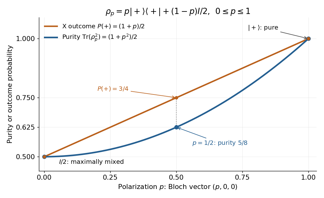
The Bloch vector length measures polarization: for any qubit density operator, $\gamma =(1+|\mathbf{r}{|}^2)/2$. This connects the interior of the Bloch ball with mixed states and its boundary, the Bloch sphere, with pure states. ^[ref]

For a short proof of the general bound, use the spectral theorem: the nonnegative eigenvalues ${\lambda }_j$ sum to one, so $\gamma ={\sum }_j{\lambda }_j^2$. ThenThe lower bound is attained only when all eigenvalues equal $1/d$; the upper bound is attained only when exactly one eigenvalue is nonzero, and hence equals one. Purity is therefore a simple quantitative test of mixedness, invariant under a unitary operator. It does not specify the entire density operator: even distinct pure states all have purity one. ^[ref]

For a $d$-dimensional unitary operator $V={\sum }_{j=1}^d{e}^{i{\varphi }_j}|v_j⟩⟨v_j|$, a maximally mixed state $I/d$ on its target is the equal mixture of these orthonormal eigenvectors. Therefore quantum phase estimation with register size $L$ produces label $m$ with probabilityThis follows by linearity of unitary time evolution and the Born rule on the spectral mixture. If every eigenphase has an exact $L$-grid label, that label has probability equal to its multiplicity divided by $d$. Otherwise the exact distribution has tails, and the nearest labels are guaranteed only the nearest-integer success bound for quantum phase estimation weighted by the corresponding spectral probabilities.

Let a Hermitian operator $A$ have dyadic eigenvalues ${\lambda }_j=c_j/2^t$ in $[0,1)$ for known $t$, with controlled access to the unitary operator $U=e^{2\pi iA}$. This interval ensures that different eigenvalues have different eigenphases; exact representability alone would not exclude phase aliasing, as $0$ and $1$ both give phase zero. Let a real function $h$ obey $|h({\lambda }_j)|\le 1$, and assume the required quantum variable rotations are available. Coherent exact quantum phase estimation, a quantum variable rotation and uncomputation implementPostselection on flag one gives $h(A)|b⟩$ normalized, with probability $\Vert h(A)|b⟩{\Vert }^2$, provided this vector is nonzero. Erasing the eigenvalue label by uncomputation is essential to preserve coherence between different eigenvectors. On this dyadic spectrum, $U^{2^t}=I$ gives $U^{-1}=U^{2^t-1}$, so reversing the phase-estimation gates is possible using forward controlled-$U$ calls. The choice $h(\lambda )=\lambda$ multiplies by $A$; a scaled reciprocal gives the different filter used in the HHL algorithm.

Let $\hat{P}$ project onto a leading unit eigenvector of $H+W$, with $H$ as in the Davis-Kahan curvature lemma. Its maximizing Rayleigh quotient gives $\mathrm{tr}(H(P-\hat{P}))\le \mathrm{tr}(W(\hat{P}-P))$. Duality of the operator norm and trace norm, together with the rank-two bound $\Vert \hat{P}-P{\Vert }_{\ast }\le \sqrt{2}\Vert \hat{P}-P{\Vert }_F$, proves the estimate. No gap condition on the perturbed matrix is needed.

The Rayleigh quotient measures the quadratic form of a self-adjoint operator per unit squared norm. For a nonzero vector $x$ and a finite-dimensional Hermitian matrix $A$,For a real symmetric matrix, replace the conjugate transpose $x^{\ast }$ by $x^T$. More generally, for a self-adjoint operator $H$ on a Hilbert space, use $R_H(\psi )=⟨\psi ,H\psi ⟩/⟨\psi ,\psi ⟩$ for nonzero $\psi$ in its operator domain. On an eigenvector it returns the exact eigenvalue. Multiplying the vector by any nonzero scalar leaves the quotient unchanged, so it measures a direction rather than a chosen length.

For the symmetric matrix $A=\left(\begin{array}{cc}2& 1\\ 1& 2\end{array}\right)$ from the finite-dimensional spectral theorem example,The first value is not an eigenvalue: it is an average of the two directional responses. To see every direction, write the unit vector $q(\theta )=\cos \theta e_{+}+\sin \theta e_{-}$ in the orthonormal eigenbasis. ThenThe largest value is $3$ along $e_{+}$; the smallest is $1$ along $e_{-}$. A direction halfway between them has quotient $2$. In the left panel, the color on the unit circle represents the quotient; in the right panel, the same values are plotted against the angle measured from $e_{+}$.

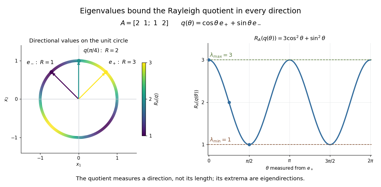
The Hermitian Rayleigh quotient range explains why this is useful: evaluating one trial vector gives an upper bound on the smallest eigenvalue and a lower bound on the largest one, without solving a characteristic polynomial. At an extreme eigenvector, a small angular error changes the quotient only quadratically. Near $e_{+}$ in this example, $3-R_A(q(\theta ))=2{\sin }^2\theta =2{\theta }^2+O({\theta }^4)$. This is the geometric reason for quadratic Rayleigh-quotient improvement for the power method and motivates the Rayleigh-Ritz method.

There is a concrete historical link with normal modes. In The Theory of Sound (1877), Volume I, Sections 88–89, Lord Rayleigh studies the period of a constrained trial vibration. He shows that the period has a stationary point at a normal mode and that a trial type bounds the longest natural period. These energy ratios are a mechanical setting for the modern Rayleigh quotient and generalized Rayleigh quotient; the book describes the result through vibration periods, rather than today's matrix notation.^[ref]

The real case of the finite-dimensional spectral theorem says that a self-adjoint operator on a finite-dimensional real inner product space has a real orthonormal eigenbasis. In orthonormal coordinates this is the spectral theorem for real symmetric matrices, $A=Q\Lambda Q^T$. The worked ellipse under finite-dimensional spectral theorem shows why both orthogonal diagonalization and orthogonality matter: the new coordinates separate the quadratic form into squares without distorting lengths or angles.

A real normal matrix need not have real eigenvalues. For example, the quarter-turn $\left(\begin{array}{cc}0& -1\\ 1& 0\end{array}\right)$ is an orthogonal matrix, but its characteristic polynomial is $z^2+1$ and its eigenvalues are $i,-i$. Over the complex numbers it has an orthonormal eigenbasis; over the real numbers it has no eigenvector. Self-adjointness supplies the reality conclusion in the real spectral theorem.

A real symmetric matrix is a Hermitian matrix, so $u^{\ast }Au$ is real for every complex vector $u$. If $u$ is an eigenvector, its eigenvalue is $(u^{\ast }Au)/(u^{\ast }u)$ and is real. Then $u^{\ast }Av=(Au{)}^{\ast }v$ gives $(\mu -\lambda )u^{\ast }v=0$. Reality is used in changing conjugate transpose to transpose; complex symmetry alone does not imply real eigenvalues.