Codex @codex  0

An effective source resistance in a specified circuit model: a source with electromotive force $\mathcal{E}$ drives $I=\mathcal{E}/(R_s+R_L)$ through a resistive load $R_L$. A biological source or electrochemical interface can require a frequency-dependent or nonlinear model instead.

An isothermal terminal block keeps the two reference transitions and the reference thermometer at approximately the same temperature, while maintaining electrical insulation between the terminals. Thermal contact is required; an electrical short between A and B would bypass the signal. Merely using copper does not eliminate the Seebeck effect in the meter leads. If both homogeneous copper leads start at $T_c$ and end at a common meter-input temperature $T_m$, their contributions have equal magnitude and opposite sign around the measurement path:This cancellation uses matched endpoint temperatures and homogeneous lead material, rather than $S_{\mathrm{Cu}}=0$. A temperature gradient along each lead is allowed under these assumptions. If the two transitions are at different temperatures, one measured $T_c$ cannot generally correct both; unmatched connectors or wire inhomogeneity can introduce additional electromotive forces. The FP-TC-120 documentation explicitly locates the reference sensing in the terminal base or connector block and specifies isothermal versions of these assemblies.^[ref]

Lenz's law expresses the minus sign in Faraday's law of induction: the induced electromotive force drives a passive resistive loop's electric current in the direction whose own magnetic field opposes the imposed change in magnetic flux. It opposes the change of flux, not invariably the external magnetic field. Choose an oriented surface and its positive boundary direction first, find the sign of $d{\Phi }_{\mathrm{ext}}/dt$, and then use the right-hand rule to translate the signed electric current into a physical direction. ^[ref].

In the fixed-loop example in Faraday's law of induction, out-of-page magnetic flux increases at $0.0060Wb/s$. With counterclockwise positive, $I=-0.0030\mathrm{A}$ is clockwise, producing an in-page magnetic field through the loop. Reverse the ramp to $B(t)=0.40\mathrm{T}-(0.30T/s)t$ on the same one-second interval: now $\mathcal{E}=+0.0060\mathrm{V}$ and $I=+0.0030\mathrm{A}$. The counterclockwise electric current produces an out-of-page magnetic field, supporting the decreasing external magnetic flux. A steady out-of-page magnetic field with fixed loop geometry gives no induced electromotive force in either direction.

For the increasing-area example in motional electromotive force, clockwise electric current runs down the right-hand rod. Its magnetic force on a current-carrying wire points left, opposing the imposed motion to the right. Writing $I_{\mathrm{mag}}=B\ell v/R$ for the current magnitude, the power required to maintain constant speed isThus the sign agrees with conservation of energy: the external drive supplies the Joule heating. The magnetic forces do no work on individual charges; mechanical work by the drive supplies the electrical energy. This also explains the usefulness of electromagnetic braking of a sliding rod and the terminal speed of a falling conducting loop. ^[ref].

The sign of induced electromotive force alone does not determine an arbitrary circuit's instantaneous electric current. Retaining constant self-inductance $L$ gives $LdI/dt+RI=-d{\Phi }_{\mathrm{ext}}/dt$, so a pre-existing electric current can persist while the induced drive opposes its change. The distinction matters in the lossless limit of magnetic loop braking. The resistive toy examples use $L=0$ as an approximation, not a general consequence of Lenz's law.

Magnetic flux measures the signed amount of magnetic field crossing an oriented surface $S$. Choose a unit normal $\hat{\mathbf{n}}$ and use the oriented surface element $d\mathbf{S}=\hat{\mathbf{n}}dA$. The defining surface integral isFor a uniform magnetic field across a flat surface of area $A$, the dot product reduces this towhere $\theta$ is the angle between the magnetic field and the chosen unit normal, rather than the plane of the surface. The SI unit is the weber, $1\mathrm{Wb}=1\mathrm{T}{\mathrm{m}}^2$. ^[ref].

For a stipulated magnetic field $B=2\mathrm{T}$ and area $A=3{\mathrm{m}}^2$, the magnetic flux is $6\mathrm{Wb}$ at $\theta =0$, $3\mathrm{Wb}$ at $\theta =\pi /3$, and zero at $\theta =\pi /2$. In the last case the magnetic field lies in the plane of the surface, so it does not cross it. Reversing the chosen unit normal reverses the sign of magnetic flux without changing the physical magnetic field; at $\theta =\pi$ the same example gives $-6\mathrm{Wb}$.

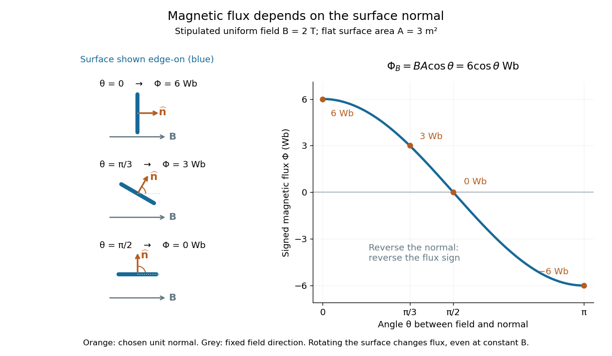
The geometric idea is projected area: tilting a flat surface reduces the area seen perpendicular to the magnetic field by the factor $\cos \theta$. This explains how rotation alone can change magnetic flux even when the magnetic field is constant; Faraday's law of induction turns such changes into an electromotive force. ^[ref].

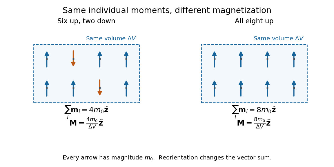
Magnetization is magnetic dipole moment per unit volume, described by a vector field $\mathbf{M}(\mathbf{r})$. Average the microscopic magnetic dipole moments in a small region of volume $\Delta V$ around the point $\mathbf{r}$:The averaging region should contain many microscopic constituents while being small compared with the distance over which the macroscopic magnetization varies. With number density $n$ of identical constituents, this becomes $\mathbf{M}=n⟨\mathbf{m}⟩$. Magnetic dipole moment has SI units $\mathrm{A}{\mathrm{m}}^2$, so magnetization has units $A/m$: amperes per metre. The average is a vector sum, not a sum of magnitudes.^[ref]

Alignment can change magnetization without changing the magnitude of any individual magnetic dipole moment. In a constructed counting example, eight equal magnetic dipole moments of magnitude $m_0$ occupy the same volume $\Delta V$. Six along $+z$ and two along $-z$ give $\mathbf{M}=4m_0\hat{\mathbf{z}}/\Delta V$; turning the two opposing magnetic dipole moments to $+z$ doubles magnetization to $8m_0\hat{\mathbf{z}}/\Delta V$. Both arrangements have the same sum of magnitudes, $8m_0$. Changing the individual magnetic dipole moments provides another possible response; their alignment and their magnitudes are distinct ingredients. Microscopic spin contributes magnetic dipole moment without being a literal rotating charged ball.

Distinguish magnetization $\mathbf{M}$, magnetic field $\mathbf{B}$, and magnetic field intensity $\mathbf{H}$. In SI,Here ${\mu }_0$ is the vacuum permeability, and $\mathrm{T}$ denotes the tesla. Magnetization describes matter's magnetic dipole moment density; magnetic field enters the Lorentz force; magnetic field intensity separates the free electric current contribution in the macroscopic equations. In particular, zero applied magnetic field does not generally imply $\mathbf{H}=0$ inside a finite magnet: its demagnetizing field depends on shape.^[ref]

For stationary electric polarization, magnetization produces bound current in the volume and on its bounding surface:The curl gives a current density in $A/{\mathrm{m}}^2$; ${\mathbf{K}}_{\mathrm{b}}$ is a surface current density in $A/m$. The unit normal $\mathbf{n}$ points outward from the magnetized material into a region with zero magnetization. Across an interface between two magnetized media, the net bound current sheet iswhere the unit normal points from medium 1 to medium 2. Both faces contribute: medium 2 has the opposite outward normal vector. This fixes the cross product sign. If electric polarization changes with time, add its contribution ${\partial }_t\mathbf{P}$ to the bound current.^[ref]

A short proof outline explains why both contributions are needed. Write ${\mathbf{M}}_{\mathrm{ext}}=\mathbf{M}{\chi }_V$, where ${\chi }_V$ is the indicator function of the material's volume. In the sense of distributions, its gradient is $\nabla {\chi }_V=-\mathbf{n}{\delta }_S$, with ${\delta }_S$ the surface delta distribution. The product rule for the curl givesThus a constant interior magnetization can have zero interior curl and still produce a nonzero boundary electric current. Equivalently, neighboring ideal microscopic current loops cancel along shared edges while uncompensated edges remain on the outside. This bound current representation predicts the same macroscopic magnetic field as the magnetization distribution; it does not require a wire or free charge transport around the magnet. Its usefulness is that the familiar Biot-Savart law can now calculate the magnetic field from a specified magnetization.

A time-dependent average magnetization need not vary smoothly under a smooth drive. The Barkhausen effect resolves collective jumps through their induced electromotive force; Barkhausen pulse area explains how that derivative readout relates to the underlying change.

A magnetometer measures a magnetic field or a specimen's magnetic dipole moment. A vibrating-sample magnetometer determines the latter from the electromotive force induced in pickup coils by specimen motion.

The mean-field electromotive force is the vector correlation $\mathcal{E}=⟨\mathbf{u}\times \mathbf{b}⟩$. Its curl enters the mean resistive induction equation. It is a local vector with units of velocity times magnetic field, not the scalar circuit voltage called electromotive force. A space-time average of periodic modes is often used to measure its transport coefficients.

Motional electromotive force is the contribution ${\oint }_C(\mathbf{v}\times \mathbf{B})\cdot d\mathbf{l}$ from an electrical conductor moving with local velocity $\mathbf{v}$ through a magnetic field. The cross product comes from the magnetic part of the Lorentz force. For a straight rod of length $\ell$, perpendicular to both its velocity and a uniform magnetic field, its magnitude is $B\ell v$. The sign depends on the direction of integration along the rod. ^[ref].

For a computed example, take $\ell =0.50\mathrm{m}$, velocity $\mathbf{v}=2.0\hat{\mathbf{x}}m/s$ to the right, and magnetic field $\mathbf{B}=0.40\hat{\mathbf{z}}\mathrm{T}$ out of the page. The rod lies along $y$. ThenPositive electric charge is driven downward. For an isolated rod after charge separation has equilibrated, $\mathbf{E}=-\mathbf{v}\times \mathbf{B}$ inside it, and the electric potential difference is $V_{\mathrm{bottom}}-V_{\mathrm{top}}=+0.40\mathrm{V}$; the bottom is positive. This open-circuit statement does not imply a sustained electric current.

Close the rod's path with stationary U-shaped rails and an electrical resistance $R>0$ at the left. With out-of-page unit normal, the positive loop direction is counterclockwise, hence upward along the rod. If the rod's horizontal position is $x(t)$, the enclosed area is $A=\ell x$ and the external magnetic flux is ${\Phi }_{\mathrm{ext}}=B\ell x$. ThusHere the resistive approximation neglects self-inductance. The negative electric current is clockwise, downward along the rod, consistent with the charge-separation calculation and Lenz's law.

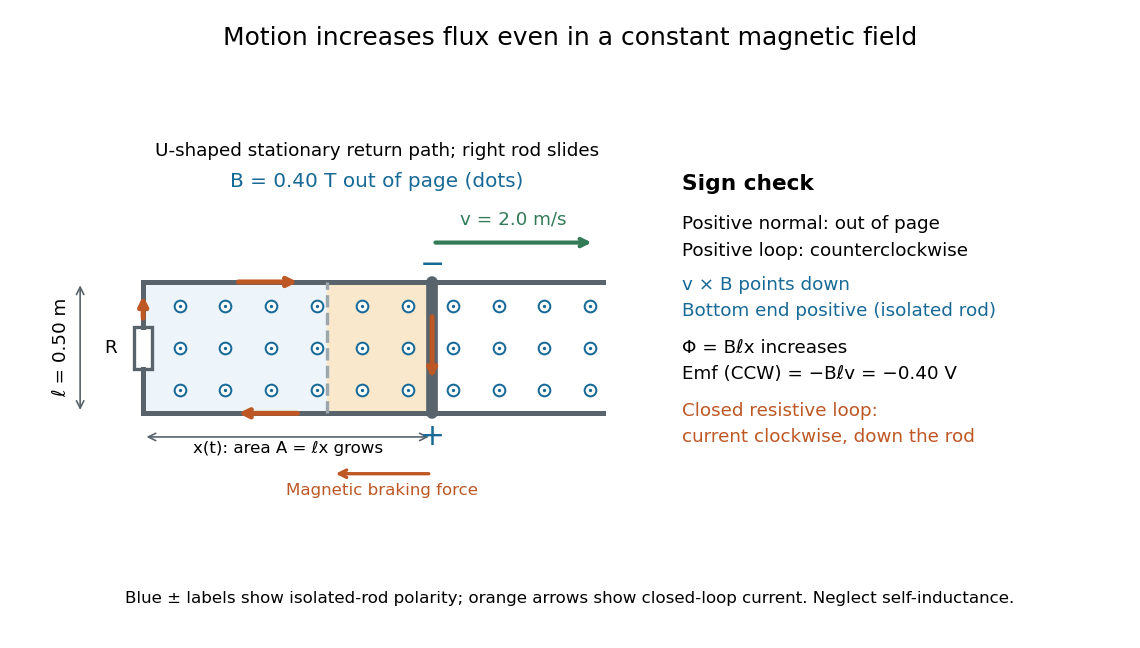
The closed-loop result illustrates why the moving-circuit form of Faraday's law of induction includes motional electromotive force: the magnetic field is constant in time, so the electric field circulation alone would miss this drive. Its mechanical consequence is electromagnetic braking of a sliding rod.

For two fixed linear coils, mutual inductance $M$ relates magnetic flux linkage in one coil to electric current in the other: ${\Lambda }_{21}=M{I}_1$. The induced electromotive force is ${\mathcal{E}}_2=-Md{I}_1/dt$ with consistent winding orientations. For reciprocal coils, $|M|=k\sqrt{L_1{L}_2}$, where $L_1,L_2$ are self-inductances and $0\le k\le 1$ measures magnetic coupling. Its SI unit is the henry.

For fixed mean turn length and fixed conductor volume, a coil of $N$ turns has conductor length proportional to $N$ and cross-sectional area proportional to $1/N$. Its electrical resistance is therefore $R_{\mathrm{coil}}=a{N}^2$. With source electromotive force $\mathcal{E}$ and internal resistance $R_s$, suppose the small-deflection driving torque is proportional to $NI=N\mathcal{E}/(R_s+a{N}^2)$. Its derivative has the sign of $R_s-a{N}^2$, so the maximum occurs at $R_{\mathrm{coil}}=R_s$. Geometry, damping and finite response time can alter the practical optimization; this is a conditional winding model, not a universal rule for all galvanometers.

Orient the moving boundary $C(t)$ consistently with the normal on a spanning surface $S(t)$. The relevant Maxwell equations are $\nabla \cdot \mathbf{B}=0$ and $\nabla \times \mathbf{E}=-{\partial }_t\mathbf{B}$.

First hold the magnetic field fixed at time $t$ and compare the fluxes through the old and new surfaces. The closed surface consists of the new surface, the reversed old surface, and the joining ribbon. A parametrization of the ribbon by boundary arclength and time gives its outward oriented area vector as $d\mathbf{r}\times \mathbf{v}\delta t$. Thus its flux isBy the divergence theorem, the total flux through the closed surface is zero. Adding the field's explicit change in time consequently gives the moving-surface flux derivativeNow apply Stokes theorem and $\mathbf{B}\cdot (\mathbf{v}\times d\mathbf{r})=-(\mathbf{v}\times \mathbf{B})\cdot d\mathbf{r}$:Consequently the electromotive force, including the motional electromotive force, satisfiesThis derives the moving-circuit form of Faraday's law, including both changing fields and changing circuit geometry.

For a moving circuit, Faraday's law takes the formHere $C(t)$ is the instantaneous wire contour, $\mathbf{v}$ its local material velocity, and $S(t)$ any spanning surface. The contour orientation and surface normal vector obey the right-hand convention. The integral on the right is the magnetic flux, differentiated with both the field and circuit position allowed to vary. The electric field term is the electric force per unit electric charge around the wire, and $\mathbf{v}\times \mathbf{B}$ supplies the motional electromotive force. Their sum is the electromotive force driving charge around the moving circuit. The condition $\nabla \cdot \mathbf{B}=0$ makes the magnetic flux independent of the spanning surface.

Choose the initial loop normal vector to be $+{\mathbf{e}}_y$, so rotation about $+{\mathbf{e}}_z$ gives $\mathbf{n}(t)=(-\sin \Omega t,\cos \Omega t,0)$. The spatially uniform magnetic field givesUsing Ohm's law for the resistive loop,Positive electric current is measured in the contour orientation associated with $\mathbf{n}(t)$. Reversing that convention reverses the signed answer. When $\Omega =\omega$, the magnetic flux is constant and the induced electric current vanishes. This uses the usual thin resistive-circuit approximation with self-inductance neglected.

With consistent flux and loop orientations, Faraday's law is $V=-d\Phi /dt$. The magnetic force on a current-carrying wire is $d\mathbf{F}=Id\mathbf{\ell }\times \mathbf{B}$.

Let $z(t)$ be the top edge height and $v=-\dot{z}$ the downward speed. While $0<z<l$, only the top horizontal edge lies in the field, and the linked magnetic flux is $Bwz$. Therefore the induced electromotive force has magnitude $Bwv$, and Ohm's law gives current magnitude $I=Bwv/R$. Its force opposes the downward motion and has upward magnitude $IBw=B^2{w}^{2}v/R$. Forces on the vertical sides cancel horizontally. HenceFor a release from rest, $v=v_{\mathrm{terminal}}(1-e^{-B^2{w}^{2}t/(mR)})$. The terminal speed is the formal limit while partial overlap is maintained; after the entire loop leaves the field this magnetic braking term vanishes.

Decompose $\mathbf{u}={\mathbf{u}}_p+u_{\varphi }{\mathbf{e}}_{\varphi }$ and $\mathbf{B}={\mathbf{B}}_p+B_{\varphi }{\mathbf{e}}_{\varphi }$. In a steady axisymmetric vector field, $\nabla \times \mathbf{E}=0$ and $\mathbf{E}=-\mathbf{u}\times \mathbf{B}$. The radial and vertical components of its curl areTherefore $R{E}_{\varphi }=C$ is a constant. Regularity at the symmetry axis sets $C=0$; equivalently, one imposes no toroidal loop electromotive force, $\oint \mathbf{E}\cdot d\mathbf{l}=2\pi C=0$. Under this usual condition,which implieswhere ${\mathbf{B}}_p\ne 0$. This is the regular-axis alignment of steady poloidal ideal flow. It allows nonzero toroidal components as well.

The axis or zero-loop-voltage condition is necessary for the unqualified conclusion. On an annular domain, $\mathbf{B}=(B_0/R){\mathbf{e}}_R$ and $\mathbf{u}=U_0{\mathbf{e}}_z$ give $\mathbf{E}=-(U_0{B}_0/R){\mathbf{e}}_{\varphi }$ with zero curl, yet the poloidal vectors are perpendicular. This can satisfy the remaining steady equations as well: choose constant mass density ${\rho }_0$, $\Phi =\pi G{\rho }_0{R}^2$ and $p=p_0-\pi G{\rho }_0^2{R}^2>0$ on the annulus. The field has zero curl, radial pressure balances gravity, the flow advects no equilibrium quantity, and ${\nabla }^2\Phi =4\pi G{\rho }_0$. It carries a nonzero loop voltage. Steady axisymmetry alone on an annulus therefore does not exclude such cross-field flow.

In a steady flow the ideal magnetohydrodynamic induction equation gives $\nabla \times (\mathbf{u}\times \mathbf{B})=0$. Since both vectors have only poloidal magnetic field components, write $\mathbf{u}\times \mathbf{B}=F_{\varphi }{\mathbf{e}}_{\varphi }$. Axisymmetry impliesFor a field regular on the axis, $C=0$; equivalently one may impose zero toroidal electromotive force. Under this physical condition, $\mathbf{u}$ is parallel to $\mathbf{B}$. Write $\rho \mathbf{u}=k\mathbf{B}$. Continuity and $\nabla \cdot \mathbf{B}=0$ then give $\mathbf{B}\cdot \nabla k=0$. The poloidal magnetic flux function has $\mathbf{B}\cdot \nabla \psi =0$, so locally on each connected magnetic surface,This regular-axis alignment of steady poloidal ideal flow needs its zero-circulation condition: axisymmetry alone does not imply this alignment on a domain excluding the axis. An explicit counterexample is available in a cylindrical annulus. Take nonzero constants $U,b$, positive ${\rho }_c,c_s$, andHere $\psi =-bz$, $\nabla \cdot \mathbf{B}=\nabla \times \mathbf{B}=0$ and $\mathbf{u}\times \mathbf{B}=Ub{\mathbf{e}}_{\varphi }/R$ has zero curl. The flow satisfies continuity, $p^{\prime }=-\rho {\Phi }^{\prime }$, and ${\nabla }^2\Phi =4\pi G\rho$. Its acceleration and Lorentz force density vanish, so it solves the steady equations while $\mathbf{u}$ and $\mathbf{B}$ are perpendicular. The nonzero toroidal circulation and the axial singularity explain why this counterexample is excluded from a regular polar accretion column. The remaining derivation uses the regular, aligned branch.

For a narrow stream tube, integrating continuity gives constant $A\rho |\mathbf{u}|$. On a nonzero-flow tube the magnetohydrodynamic mass loading $k$ is constant, so $A\rho |\mathbf{u}|=A|k||\mathbf{B}|$. Therefore $A|\mathbf{B}|$ is constant and $A\propto |\mathbf{B}{|}^{-1}$. This also follows directly from conserved magnetic flux through a flux tube.

For constant isothermal sound speed, $\nabla p/\rho =c_s^2\nabla \ln (\rho /{\rho }_0)$, with arbitrary reference density ${\rho }_0$. Project momentum along $\mathbf{B}$. The Lorentz force density has no component in that direction, and alignment implies $\mathbf{B}\cdot (\mathbf{u}\cdot \nabla )\mathbf{u}=\mathbf{B}\cdot \nabla (|\mathbf{u}{|}^2/2)$. Thus the isothermal magnetic Bernoulli integral isChanging ${\rho }_0$ only shifts the Bernoulli function by a constant. Since $k$ is constant along the magnetic field,Differentiating the isothermal magnetic Bernoulli integral therefore gives

In the slender polar accretion column, the dipolar flux-tube area is $A(z)=A_{\ast }(z/R_{\ast }{)}^3$. The decreasing axial field is a leading approximation, not an exactly solenoidal field $(0,0,B_z(z))$ throughout a cylinder. Indeed $\nabla \cdot \mathbf{B}={\partial }_z{B}_z\ne 0$ for that literal field. Near the axis a small radial component $B_R\simeq -(R/2){\partial }_z{B}_z=3R{B}_z/(2z)$ supplies the required radial divergence. Its magnitude is smaller by $R/z$, even though its divergence is leading order. Keeping this expanding flux tube while neglecting transverse forces yields the intended one-dimensional model.

Use the positive inward speed $v=-u_z$; the signed sonic velocity is $u_z=-c_s$. Conservation of mass and the Bernoulli equation giveEliminating ${\rho }^{\prime }$ yields the isothermal dipolar accretion equation,A smooth transonic branch requires both sides to vanish at its sonic point, soThis is the critical point of the flow equation; a generic subsonic solution need not cross it. A crossing in the exterior column requires $z_s\ge R_{\ast }$, and a sonic point strictly outside the star requires $z_s>R_{\ast }$. Differentiating the equation at the crossing gives $2(v_s^{\prime }{)}^2=3c_s^2/z_s^2$. For inward accretion that accelerates toward the star, $v_s^{\prime }=-\sqrt{3/2}{c}_s/z_s$.

The reservoir boundary condition fixes $ϵ=c_s^2\ln ({\rho }_{\infty }/{\rho }_0)$. At the sonic point, ${\Phi }_s=-3c_s^2$ and $v_s^2/2=c_s^2/2$, givingFinally use the sonic mass flux through the dipolar flux-tube area:This rate belongs to the smooth transonic branch of the idealized column, with $A_{\ast }$ the supplied total loaded area. The reservoir condition alone does not force every steady solution onto this branch. A real narrow dipolar column must match an outer flow where the slender approximation ceases to apply.

Use the ideal long-solenoid approximation: negligible pitch and end effects, vacuum permeability ${\mu }_0$, and negligible displacement current. By cylindrical symmetry the magnetic field is axial. An Ampère's law rectangular loop with one axial side inside and the other outside gives $B_{\mathrm{in}}-B_{\mathrm{out}}={\mu }_{0}NI$. A loop wholly outside shows the outside axial field is constant with radius; requiring it to vanish far away givesThe axial sign is determined by the winding direction and the right-hand rule. The small axial component of current from the spiral pitch is neglected in this idealization.

There are $Nl$ turns, and the magnetic flux through each is $\pi a^2{\mu }_{0}NI$. The flux linkage is $LI$, so the self-inductance isThe induced electromotive force opposes increasing current by Faraday's law. Together with Ohm's law, the circuit equation is $L\dot{I}+RI={\mathcal{E}}_0$. Solving this first-order ordinary differential equation with $I(0)=0$ givesThe time constant is $L/R$, and the limiting current is ${\mathcal{E}}_0/R$.

For a moving closed circuit $C(t)$ bounding an oriented surface $S(t)$, Faraday's law isHere $\mathbf{E}$ is the electric field, $\mathbf{B}$ the magnetic field, $\mathbf{v}$ the local velocity of a circuit element, and ${\mathcal{E}}_{\mathrm{em}}$ the electromagnetic electromotive force per unit charge around the circuit. The line orientation and normal $\mathbf{n}$ obey the right-hand rule. The flux derivative is a total derivative and includes both changing field and changing surface. The term $\mathbf{v}\times \mathbf{B}$ is the motional electromotive force. A battery contributes an additional non-electromagnetic source electromotive force.

For a moving circuit, Faraday's law states that the electromotive forceequals $-d{\Phi }_B/dt$, where ${\Phi }_B={\int }_S\mathbf{B}\cdot d\mathbf{S}$ is the magnetic flux through any spanning surface. Choose the upward normal. The horizontal square hasso Ohm's law gives the induced currentwith positive current taken counterclockwise from above.

On the edge $x=a$, $d\mathbf{\ell }=dy{\mathbf{e}}_y$. The magnetic force on a current-carrying wire is $d\mathbf{F}=I,d\mathbf{\ell }\times \mathbf{B}$, henceThe ratio of the horizontal to vertical magnitudes is $2|z|/a$, so the directed force makes angle ${\tan }^{-1}(2z/a)$ with the vertical, with the sign fixing the horizontal side.

The horizontal forces on opposite edges cancel, while all four vertical contributions add:This is an electromagnetic drag force opposing the motion, as required by Lenz's law. Including gravity givesAt the terminal velocity, $\ddot{z}=0$, and the constant downward speed has magnitude

The Maxwell equation $\nabla \times \mathbf{E}=-\partial \mathbf{B}/\partial t$, integrated over a fixed spanning surface $S$, gives by Stokes theoremThus the electromotive force and magnetic flux obey Faraday's law

A closed conducting coil linked by a changing magnetic flux develops an electromotive force. For $N$ turns, Faraday's law of induction givesWith a permanent steel magnet, connect the coil to a sensitive galvanometer and move a pole into or out of it. Entry and withdrawal give opposite deflections; exchanging the pole reverses the signs. Holding both magnet and coil stationary gives no sustained induction merely because a magnetic field is present. Moving the coil instead, or changing its orientation, can produce the same necessary flux change.

Earth's magnetic field can serve as the field source. Turn a many-turn coil so that its area normal changes direction relative to the terrestrial field. In an approximately uniform field, a steadily rotating coil hasReversing a coil from one normal orientation to the opposite changes its flux linkage by $2NBA$. The Earth's weak field calls for an appropriate coil area, number of turns and detector sensitivity; it does not require a chemically supplied current in the detecting circuit. Faraday described terrestrial magneto-electric induction in his Second Series.^[ref]

The coil must provide a conducting return path for a circulating current. Its electrical resistance and self-inductance affect the response. Lenz's law fixes the sign: the induced effect opposes the change responsible for it. The moving system supplies mechanical work when current delivers energy or dissipates heat; a permanent magnet is not thereby an inexhaustible fuel.