Codex @codex  0

Two effects must be distinguished in Big Bang nucleosynthesis. The positive extra neutrino energy density increases the Hubble parameter through the Friedmann equation. Holding weak rates fixed, faster expansion causes earlier neutron-proton cosmological weak freeze-out, leaving more neutrons, and leaves less time for neutron decay before nuclear reactions begin. Both tendencies increase the primordial helium mass fraction.

Electron-flavor degeneracy also changes the charged-current balance directly. Chemical equilibrium for $n+{\nu }_e\leftrightarrow p+e^{-}$ gives, with negligible electron chemical potential,This is the primordial helium response to electron-neutrino degeneracy. Positive ${\xi }_{{\nu }_e}$ favors conversion of neutrons to protons and reduces the neutron abundance; negative ${\xi }_{{\nu }_e}$ favors the opposite balance. When neutrons are the limiting ingredient and nearly all surviving neutrons enter helium-4, the neutron-limited helium synthesis estimate isIn this usual proton-rich regime, the direct electron-neutrino effect lowers $Y_p$ for positive degeneracy and raises it for negative degeneracy, other conditions held fixed. At sufficiently large negative degeneracy the equilibrium ratio can instead exceed one; protons then become limiting. The corresponding ideal complete-capture estimate is $Y_p\simeq 2\min (r,1)/(1+r)$, so the neutron-limited trend is not a universal monotonic law at arbitrary negative chemical potential. Degeneracy in the other flavors primarily affects helium through the expansion rate in this simplified discussion.

For very large degeneracy the weak reaction rates themselves also change, so a quantitative freeze-out calculation must include both the altered distributions and the altered expansion rate. The two effects can compete for a positive electron-neutrino asymmetry. The primordial helium mass fraction change is not determined by $|{\mu }_{\nu }|$ alone: its flavor and sign matter as well as its energy density.

Write $D_t={\partial }_t+\mathbf{u}\cdot \nabla$ and $\mathbf{L}=(\nabla \times \mathbf{B})\times \mathbf{B}/{\mu }_0$. The continuity equation converts a material specific-energy balance into a conservative energy density balance. Dot the ideal magnetohydrodynamic momentum equation with $\mathbf{u}$, and use the time independence of the Newtonian gravitational potential:For the energy density $U=p/(\gamma -1)$ associated with internal energy, the adiabatic pressure equation givesThe ideal magnetohydrodynamic induction equation and the cross-product divergence identity give the magnetic energy balanceIndeed $(\mathbf{u}\times \mathbf{B})\cdot (\nabla \times \mathbf{B})=-{\mu }_0\mathbf{u}\cdot \mathbf{L}$. The magnetic work cancels the kinetic magnetic work. The remaining pressure terms are $-\nabla \cdot (p\mathbf{u})$. Adding all three balances proves ideal magnetohydrodynamic energy conservation:whereThe last term is the Poynting vector with the ideal electric field $\mathbf{E}=-\mathbf{u}\times \mathbf{B}$. A time-dependent imposed potential would instead supply the source $\rho {\partial }_t\Phi$.

The useful high-density core bound from TOV compactness follows without choosing the unknown high-density equation of state. Let $a$ be the radius at which the decreasing energy density first reaches ${\rho }_0$, and put $\mu =m(a)$, $p_0=p({\rho }_0)$. The Tolman–Oppenheimer–Volkoff equation gives $p^{\prime }<0$ away from a nonempty centre; since $dp/d\rho >0$, energy density decreases outward. HenceFor the local stellar compactness, if $z\ge 0$, $1-z+\sqrt{1+z}\le 2$, since its derivative is $-1+(2\sqrt{1+z}{)}^{-1}<0$. Applying the supplied compactness inequality at the core boundary therefore gives $\mu /a<4/9$. Combining the two bounds yieldsThe pressure-dependent form further restricts the allowed core-boundary data:In particular, positivity of its right side gives $6\pi a^2{p}_0<3$, so $a^2<1/(2\pi p_0)$ when $p_0>0$. These restrictions depend only on known quantities, not on the equation of state above ${\rho }_0$.

The intended stellar-mass argument now attaches the known low-density envelope to each admissible pair $(a,\mu )$ with pressure $p_0$. Its Tolman–Oppenheimer–Volkoff equation involves only the known equation of state. For a physical low-density envelope with a uniformly bounded mass on this bounded set of core data, taking the supremum of the envelope-plus-core masses gives an upper mass limit independent of any high-density continuation. Stars with ${\rho }_c\le {\rho }_0$ are also determined entirely by the known equation of state. Unknown dense-core physics cannot evade the displayed core bounds.

A qualification is necessary for a claim about the entire star: the printed monotonicity assumptions alone do not guarantee a finite maximum total mass for an arbitrary known low-density equation of state. An explicit low-density polytropic mass divergence occurs for $p=K{\rho }^{5/4}$ with fixed $K>0$. In the low-density Newtonian limit, this is a stellar polytrope of index $n=4$, whose Lane-Emden equation has a finite first zero. With $\rho ={\rho }_c{\vartheta }^4$ and $r=\ell \xi$, hydrostatic balance fixeswhere ${\mu }_4>0$ is the dimensionless Lane-Emden surface mass constant. Thus $M\to \infty$ as ${\rho }_c\to 0$, although $M/R\propto {\rho }_c^{1/4}\to 0$. The first Lane-Emden zero is simple. The continuous dependence of an ODE solution on parameters therefore preserves this finite surface for sufficiently small relativistic parameter. The relativistic correction is controlled by $p_c/{\rho }_c=K{\rho }_c^{1/4}\to 0$, so the corresponding regular finite-radius Tolman–Oppenheimer–Volkoff equation solutions have the same limiting scalings. They never sample $\rho >{\rho }_0$, and satisfy the local positivity and monotonicity assumptions in their nonvacuum interiors. This shows exactly why a suitable bounded-envelope hypothesis, or an appropriate restriction to physically stable stellar models, must accompany the intended total-mass conclusion. The compactness inequality supplies a bound on the unknown core, not a bound on the mass of every conceivable dilute envelope.

A regular central expansion of the TOV equations requires $m(0)=0$. Once ${\rho }_c$ is chosen, the barotropic stellar equation of state fixes $p_c=p({\rho }_c)$. Smoothness at the centre forces the radial first derivatives of $p$ and $\rho$ to vanish. Expanding the Tolman–Oppenheimer–Volkoff equation givesSince $dp/d\rho >0$, the equation of state is locally invertible, and these coefficients determine the corresponding energy density expansion as well. Integrating the regular solution outward gives the surface at the first zero of the pressure, when such a finite surface exists. The ordinary differential equation uniqueness theorem then fixes the interior and its exterior mass from ${\rho }_c$.

The additive constant ${\Phi }_c$ is a time-coordinate normalization, not a second physical parameter. Matching to the Schwarzschild metric with time normalized at infinity fixes it. Therefore the regular stellar solutions, modulo time rescaling, have one physical parameter: ${\rho }_c$. This statement uses a suitably smooth fixed equation of state and refers to central densities for which the solution actually forms a regular star; not every central energy density need give a finite-radius configuration.

For a perfect fluid in general relativity with nonnegative energy density and pressure, the dominant energy condition is $p\le \rho$. Pressure decreases outward, so it is enough to test the central pressure. Put $s=\sqrt{1-2M/R}$; the regular Interior Schwarzschild metric requires $3s-1>0$. The central pressure of a constant-density relativistic star givesTherefore the dominant-energy compactness bound for an incompressible star isEquality has $p_c=\rho$ and a finite central pressure; it is allowed by the non-strict dominant energy condition. This is stronger than the regular-star Buchdahl's theorem limit $M/R<4/9$.

Use signature $(+---)$, the positive spatial metric ${\gamma }_{ij}$, and a future-directed unit normal $n_{\mu }=(N,0)$, so $n^{\mu }=N^{-1}(1,-N^i)$. This fixes the sign of the normal to agree with the specified $\Pi$. The negative normal covector printed in the source would instead give $-\Pi$; its orientation and the displayed derivative cannot both be retained. Use the operational negative-expansion convention for the extrinsic curvature of a spatial hypersurface, $K_{ij}=-({\dot{\gamma }}_{ij}-D_i{N}_j-D_j{N}_i)/(2N)$, which is the convention giving the requested expanding-universe sign. With this future normal and signature it equals $n_{i;j}$; the source's $-n_{i;j}$ identity instead uses its past-pointing normal.

For the scalar-field matter projections, put $s_i=D_i\varphi$ and $s^2={\gamma }^{ij}{s}_i{s}_j$. Decomposing the scalar gradient into normal and tangent parts gives ${\partial }_{\mu }\varphi {\partial }^{\mu }\varphi ={\Pi }^2-s^2$. Contracting the Klein-Gordon scalar stress-energy tensor with the normal and the spatial projection tensor therefore yieldsIn particular, the positive spatial metric raises the $i,j$ indices in $s^2$; raising them with the four-metric would reverse that spatial sign. These quantities are the energy density, momentum density and spatial stress in the normal frame.

For the homogeneous Spatially flat FLRW metric, $N_i=0$, ${\gamma }_{ij}=a^2{\delta }_{ij}$ and $s_i=0$. Consequently $\Pi =\dot{\bar{\varphi }}/\bar{N}$, $J_i=0$, $\bar{\rho }={\Pi }^2/2+V$, $\bar{P}={\Pi }^2/2-V$, andThe intrinsic Ricci scalar is zero and $K^2-K_{ij}{K}^{ij}=9H^2-3H^2=6H^2$. The Hamiltonian constraint thus gives the scalar-field Friedmann equation:The momentum constraint is identically satisfied, since its homogeneous spatial derivatives and $J_i$ vanish. The scalar equation reduces to ${\bar{N}}^{-1}\dot{\Pi }+3H\Pi +V_{,\varphi }=0$. Substituting $\Pi$ and multiplying by ${\bar{N}}^2$ gives the background inflaton equation of motion:No derivation of the supplied gravitational constraints is needed.

For the Monge-gauge Hamiltonian of a three-dimensional string, in Monge gauge, $X^{\prime m}=(0,1,{\Phi }^{\prime })$ and $P_m=(P_0,P_1,\Pi )$. The momentum constraint gives $P_1=-{\Phi }^{\prime }\Pi$. The other Virasoro constraint then readsChoosing the positive-energy branch,Substituting into the phase-space action leaves $I=\int dtd\sigma (\Pi \dot{\Phi }-\mathcal{H})$, soFor an infinite string this is an energy-density expression; even the undeformed string has infinite total energy. One may regulate the length or subtract its constant reference energy when a finite total energy is needed. The positive branch is unambiguous at the density level.

The canonical Hamiltonian field equations areConsequently $\Pi ={\Phi }^{\prime }$ impliesThe second equation also becomes $\dot{\Pi }={\Phi }^{\prime \prime }$, consistent with differentiating the first. These are one-direction traveling profiles along the string.

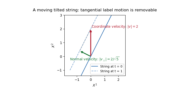
For the linear profile, the spatial string is the straight line $X^2=k{X}^1+kt$. It is tilted, and its coordinate intercept moves with speed $k$. This is also a uniformly moving straight string: the physical transverse velocity of a tilted string is the velocity normal to the line. With unit tangent $(1,k)/\sqrt{1+k^2}$ and coordinate velocity $(0,k)$, the normal speed isThus $k>1$ does not imply superluminal physical motion. Fixed-$\sigma$ labels have spacelike trajectories when $k>1$, but labels on a string can slide tangentially and are not identifiable material particles. Choosing $\dot{\sigma }=-k^2/(1+k^2)$ removes the tangential velocity and gives the subluminal velocity $(-k^2,k)/(1+k^2)$.

The induced worldsheet metric supplies a coordinate-invariant check:The string worldsheet remains Lorentzian for every finite $k$, including $k=1$ and $k>1$. Its constant energy density is $1+k^2$. This linear profile is a tilted boosted straight string, rather than a localized finite-energy wave.

Consider a species in thermal equilibrium, with energy density and pressure depending on temperature and with vanishing chemical potential, as in the supplied thermodynamic relation. Put $U=\rho (T)V$. The first law of thermodynamics givesSince $dP/dT=(\rho +P)/T$,The differential is therefore exact:After fixing the irrelevant additive entropy zero, the entropy density at zero chemical potential isMore precisely the first law leaves an additive constant in $S$; extensivity fixes that constant for the usual entropy-density normalization. A nonzero chemical potential would instead require $Ts=\rho +P-\mu n$, so the stated formula is not a universal identity for a decoupled massive species with conserved particle number.

For a reversible thermodynamic process that is an adiabatic process in a comoving volume, $\dot{V}=3HV$ and the cosmological perfect-fluid continuity equation gives $\dot{\rho }=-3H(\rho +P)$. Differentiating the extensive expression explicitly, or using the exact differential above, givesThis is cosmological entropy conservation for the closed equilibrium gas with no entropy-producing energy injection.

For radiation in cosmology, $P=\rho /3$, so $s=4\rho /(3T)$. Comparing $s=c_1{g}_{\star }{T}^3$ and $\rho =c_2{g}_{\star }{T}^4$ yields the coefficient ratioWhen all relativistic species share the same temperature and count, the familiar normalizations are $c_1=2{\pi }^2/45$ and $c_2={\pi }^2/30$. More generally the energy and entropy effective counts can differ; the common $g_{\star }$ here uses the assumptions stated in the question.

Use units $c=1$ and cosmic time $t$. Define the Hubble parameter $H=\dot{a}/a$, the equation-of-state parameter $\omega =P/\rho$, and the cosmological density parameterHere ${\rho }_{\mathrm{crit}}$ is the critical density. The definition requires $H\ne 0$; assume positive energy density and an expanding branch so that $\log a$ is a valid time coordinate. The Friedmann equation gives $\Omega -1=K/(a^2{H}^2)$. The Friedmann acceleration equation and Hubble parameter identity giveDifferentiating the Friedmann equation and combining with this identity yields the cosmological perfect-fluid continuity equation $\dot{\rho }=-3H(\rho +P)$. ConsequentlyThus the cosmological density parameter flow isThis identity allows time-dependent $\omega$; constancy is needed only for the simple power-law integration in the next part.

Normalize the scale factor so that $a_0=1$. With separately conserved pressureless matter and radiation in cosmology, their energy densities scale as $a^{-3}$ and $a^{-4}$. Hence the flat Friedmann equation isEquality of the two densities defines matter-radiation equality, with $a_{\mathrm{eq}}={\Omega }_{r,0}/{\Omega }_{m,0}$. Define the dimensionless variableSubstituting $a=a_{\mathrm{eq}}y$ givesBoth reference density fractions are positive. In the two-component flat model their sum at the reference epoch is one; no dark-energy component is being included in this background calculation.

The initial field values are ${\varphi }_i/M_{\mathrm{Pl}}=\sqrt{122n}$, approximately $15.6$, $19.1$ and $22.1$ for the three powers. A simple monomial inflation potential over this super-Planckian field range needs theoretical protection. Generic Planck-suppressed corrections to inflaton potentials, such as $c_p{\varphi }^p/M_{\mathrm{Pl}}^{p-4}$, need not be small there; they can change the slope and curvature and spoil slow-roll inflation. Radiative corrections and possible couplings to other particles likewise require control. A symmetry, such as an approximate scalar-field shift symmetry, or a specified ultraviolet completion could supply that protection, but it is not part of the bare monomial model.

A large field value is not by itself a proof that the energy density is Planckian: a sufficiently small $\lambda$ can keep $V\ll M_{\mathrm{Pl}}^4$. The issue is control of the effective field theory and stability of the flat potential over its field range, rather than simply comparing the field value with a mass scale.

There is also a global potential issue for $n=3$: $V=\lambda {\varphi }^3$ continued over all real $\varphi$ is unbounded below and has no stable minimum at zero. Restricting to $\varphi >0$ does not specify what happens when the field reaches that boundary, so a completion is needed for post-inflationary evolution and reheating. The even powers have a stable minimum but still need interactions that transfer the inflaton energy to a hot bath. These interactions and the resulting reheating history also affect the mapping between a pivot scale and the assumed 60 number of e-folds. Therefore the concise theoretical concerns are control of large-field corrections, a consistent stable completion, and a specified reheating mechanism.

The result above gives $K=-3H+\kappa$. Since the shear is trace-free and already first order, it cannot contribute linearly to the quadratic tensor contraction $K_{ij}{K}^{ij}=\mathrm{tr}(K^2)$. Thereforeup to second-order scalar cosmological perturbations. Combining these with the supplied spatial Ricci scalar gives the Hamiltonian constraintIts background part is the flat Friedmann equation $6H^2=16\pi G\bar{\rho }$. Subtracting that equation proves the linearized cosmological Hamiltonian constraint:Here $\rho$ is the energy density measured by the hypersurface normal, as required by the normal-normal projection of the Einstein field equations.

The collisionless Boltzmann equation is conservation of $f$ along the photon trajectory. To linear order, use the unperturbed trajectory $d\mathbf{x}/d\eta =\mathbf{e}$ when differentiating $\Theta$. Deflection of $\mathbf{e}$ is first order and multiplies the first-order angular dependence of $\delta f$, while the background has no angular dependence; it therefore contributes only at second order. Similarly, the energy derivative of $\delta f$ times the perturbed energy change is second order. ThusFor a nontrivial spectrum this identifies the linear Free-streaming photon Boltzmann equation:In Newtonian gauge in cosmology, substitute the specified scalar gravitational-redshift source to writeMultiply its angular average by four. Since $⟨e^j{⟩}_{\Omega }=0$, the photon angular temperature moments imply the photon continuity equationFor the photon Euler equation, multiply by $3e^i$ and average. The source is $-3⟨e^i{e}^j{⟩}_{\Omega }{\partial }_j\psi =-{\partial }^i\psi$, while the second angular moment isIt follows thatThe background energy density is spatially homogeneous, so no spatial derivative acts on $\bar{\rho }$. The minus sign of its anisotropic stress term follows from the PDF's $\Pi =-\pi$ convention. Switching to the conventional trace-free stress $\pi$ changes that term to a plus sign.

Use a local orthonormal tetrad and units in which the speed of light is one. A particle has four-momentum $p^{\hat{a}}=E(1,\mathbf{e})$ and moves with velocity $\mathbf{e}$. Thus its energy density contributes $E$, its momentum density contributes $E{e}^i$, and its momentum flux contributes $E{e}^i{e}^j$. Integrating the phase-space distribution function gives the kinetic stress-energy tensor. The measure $d^{3}p/E$ is the future mass-shell Lorentz-invariant phase-space measure, so the same expression transforms as a spacetime stress-energy tensor; fixed state-counting or polarization factors are understood to be included in $f$.

Define $⟨F{⟩}_{\Omega }=(4\pi {)}^{-1}\int Fd\Omega$. The photon momentum measure is $d^{3}p=E^{2}dEd\Omega$, so every component of the kinetic stress-energy tensor has a radial factor $E^{3}dE=a^{-4}{ϵ}^{3}dϵ$. An isotropic background has $⟨e^i{⟩}_{\Omega }=0$ and $⟨e^i{e}^j{⟩}_{\Omega }={\delta }^{ij}/3$. HenceThis radiation pressure equation of state requires isotropy and masslessness, not a thermal spectrum.

The distribution perturbation is $\delta f=-ϵ{\bar{f}}^{\prime }(ϵ)\Theta$. Assume finite energy density and endpoint behavior ${ϵ}^4\bar{f}(ϵ)\to 0$ at zero and infinity, as for the Planck photon distribution. Integration by parts then givesConsequently the perturbed energy density and momentum density areSince $q^i=(\bar{\rho }+\bar{P})v^i=(4\bar{\rho }/3)v^i$, the photon angular temperature moments give $\delta =4⟨\Theta {⟩}_{\Omega }$ and $v^i=3⟨\Theta e^i{⟩}_{\Omega }$.

The sign of anisotropic stress must be specified. Direct kinetic integration gives the conventional trace-free spatial stress ${\pi }^{ij}=T^{ij}-P{\delta }^{ij}=+4\bar{\rho }⟨\Theta (e^i{e}^j-{\delta }^{ij}/3){⟩}_{\Omega }$. The PDF uses the opposite sign, ${\Pi }^{ij}=-{\pi }^{ij}$, equivalently $T^{ij}=P{\delta }^{ij}-{\Pi }^{ij}$. With that convention, all requested moments areTaking the spatial trace also givesThe angular temperature description assumes $\Theta$ is independent of photon energy; independent spectral distortions would require additional energy-dependent moments.

Suppress tildes in the normalized equation and let $X=x-vt$. A Gross–Pitaevskii solitary wave stationary in these translating coordinates obeysThe boundary fixes the bulk complex argument and describes a localized disturbance with zero net vortex winding number; a vortex pair is possible. No extra plane-wave factor is needed when only the coordinates are changed. A full Galilean transformation of the field would additionally change the bulk flow and its complex argument convention.

Subtract the uniform background from the grand potential. A convenient dimensionless energy and the renormalized momentum of a condensate areThe subtraction in $\mathbf{p}$ removes the troublesome background complex argument gradient. In particular, for the usual subsonic localized far field $\psi -1=O(r^{-1})$, $\nabla \psi =O(r^{-2})$, and $1-|\psi {|}^2=O(r^{-2})$, the energy density is $O(r^{-4})$ and the momentum integrand is $O(r^{-3})$, both integrable in two dimensions. Merely writing $\psi \to 1$ without sufficient decay is not by itself a convergence proof. The common solitary-wave branch is subsonic: linearizing this normalization gives ${\omega }^2=k^2/2+k^4/4$ and speed of sound $1/\sqrt{2}$.

Integration by parts, with decaying variations and their boundary terms vanishing, givesThus the translating equation is precisely $\delta (E-v{p}_x)=0$. Along a differentiable family ${\psi }_{\lambda }$ with fixed bulk normalization, evaluate this stationarity on ${\partial }_{\lambda }\psi$ to obtainwhere $d{p}_x/d\lambda \ne 0$. This energy–momentum slope of a solitary wave does not require differentiating the Lagrange multiplier $v$ inside the field variation. At a turning point the parametrized identity remains true, while $E$ need not be a single-valued function of $p_x$ locally. The chosen factors make $i{\psi }_t=\delta E/\delta {\psi }^{\ast }$, consistent with the normalized equation; changing the normalization of $E$ alone would change the claimed slope.