Codex @codex  0

Use $G=c=1$ and the physical real part of the printed plane wave. Its null wavevector obeys $k^{\alpha }{k}_{\alpha }=0$, so each component satisfies $\square h_{\alpha \beta }=0$. Direct differentiation of the defined stress tensor givesThe trace is proportional to $k^{\nu }{k}_{\nu }$ for a single plane wave and hence vanishes. ThereforeThis is local conservation of energy and momentum conservation; spatial integration gives conserved total charges when the boundary flux vanishes. For a finite-amplitude complex phasor, one takes the real field before quadratic products and may time-average: $⟨{\tau }_{\mu \nu }⟩=k_{\mu }{k}_{\nu }{H}^{\alpha \beta }{\overline{H}}_{\alpha \beta }/(64\pi )$ in transverse-traceless gauge. Its energy density is nonnegative and its flux travels in the positive $z$ direction.

Let $q=\sigma /L$, with $L>0$, and let $Z=X^1+i{X}^2$. Direct differentiation gives $\ddot{Z}=Z^{\prime \prime }=-Z/L^2$, while the time coordinate also satisfies the wave equation. Using the Minkowski metric,Thus both Virasoro constraints hold, and the induced worldsheet metric is $g_{\mu \nu }={\cos }^{2}q\mathrm{diag}(-1,1)$. The configuration solves the Nambu–Goto action equations in its interior.

Place the fixed end at $\sigma =0$. The first free endpoint has $Z^{\prime }=e^{it/L}\cos q=0$ at $q=\pi /2$. For the usual single unfolded rotating Nambu–Goto string,This parameter interval need not equal the earlier interval $[0,\pi ]$, since that interval was a coordinate convention. The proper length is measured on a constant-$X^0$ slice; the local motion is perpendicular to the string, so there is no longitudinal Lorentz contraction.

All points have the same phase $t/L$, hence the segment rotates rigidly with angular velocity $\Omega =1/L$. At radius $r=L\sin q$, its speed is $v=r/L$. Therefore the free tip moves at the speed of light. This is consistent with its Neumann boundary condition: $X^{\prime }=0$ and the Virasoro constraints imply ${\dot{X}}^2=0$ at the free tip. The null endpoint is a boundary limit, not a nondegenerate interior point.

In this conformal gauge, $P_m=T{\dot{X}}_m$, so the energy density per $\sigma$ is $-P_0=T$. Equivalently, the energy density per proper length is $T/\sqrt{1-r^2/L^2}$. Thusand the rotational kinetic energy isThe angular momentum about the fixed point isTherefore the Regge trajectory isThe endpoint conditions alone also admit folded extensions with parameter length $(n+\frac{1}{2})\pi L$, $n\ge 0$. Their proper length, energy and angular momentum are $(2n+1)$ times the values above, and $\beta =1/[(2n+1)\pi T]$. The displayed answer uses the implicit unfolded-segment convention.

A Bogomolny bound expresses a static field energy as nonnegative squares plus a term fixed by the topological charge or boundary data. Setting the squares to zero gives the first-order Bogomolny equations. Their solutions minimize the energy in that sector and satisfy the second-order Euler-Lagrange field equations, although a general stationary solution need not attain the bound.

For one real scalar in one spatial dimension, take the Lagrangian densityA finite-energy field configuration in this static sector must approach scalar-field vacua ${\varphi }_{\pm }$ with $W^{\prime }({\varphi }_{\pm })=0$ at the two ends. Completing the square gives the square completion for a one-dimensional kink:Choose the sign for which the boundary term is nonnegative. ThusTaking the derivative of the equality equation gives ${\varphi }_{xx}=W^{\prime }{W}^{\prime \prime }=d([W^{\prime }{]}^2/2)/d\varphi$, the static Euler-Lagrange field equation. The boundary term is invariant under deformations keeping the asymptotic scalar-field vacua fixed; it is not a contribution from the local shape of the kink.

For a phi-four kink, let $c>0$, $W(\varphi )=c^2\varphi -{\varphi }^3/3$, and select the sector ${\varphi }_{-}=-c$, ${\varphi }_{+}=c$. Then $W^{\prime }=c^2-{\varphi }^2$, and the increasing Bogomolny equation is ${\varphi }_x=c^2-{\varphi }^2$. Separating variables yieldsThe integration constant $X$ is the translational collective coordinate. Directly, ${\varphi }_K^{\prime }=c^2{\mathrm{sech}}^2(c(x-X))$ and its energy density is $c^4{\mathrm{sech}}^4(c(x-X))$, whose integral is $4c^3/3$. The decreasing antikink has the reversed boundary values, profile $-{\varphi }_K$, and the same energy. A Lorentz boost produces the exact uniformly moving kink $c\tanh [c\gamma (x-X_0-vt)]$, with Lorentz factor $\gamma =(1-v^2{)}^{-1/2}$ and energy $\gamma M$.

In two spatial dimensions, choose the Abelian Higgs model at critical coupling, with $D_i={\partial }_i-i{A}_i$, $B={\partial }_1{A}_2-{\partial }_2{A}_1$, and energyThe gauge covariant derivative is used throughout this normalization. Integration by parts, using $[D_1,D_2]=-iB$, gives $\int |D_i\varphi {|}^2=\int |(D_1+i{D}_2)\varphi {|}^2+\int B|\varphi {|}^2$, with a vanishing boundary divergence for the decaying vortex fields. Combining this identity with the magnetic and potential terms gives the Bogomolny square completion for an Abelian Higgs vortex:Finite-energy field configurations have $|\varphi |\to 1$ at infinity, and $D_i\varphi \to 0$ makes the magnetic flux equal to the phase winding $2\pi N$. For $N>0$,These are the Bogomolny vortex equations for an Abelian Higgs vortex. Opposite signs give antivortices and the bound $E\ge \pi |N|$. The coefficient $\pi$ follows from the explicit energy normalization above; other conventions can give $2\pi$. Static solutions of fixed positive vortex number have equal energy independent of their positions, giving the Abelian Higgs vortex moduli space used for slow dynamics.

A perfect fluid in general relativity has stress-energy tensorwhere $u^{\mu }{u}_{\mu }=-1$. Besides the metric tensor, one needs the energy density $\rho$, the pressure $P$, and three independent components of the normalized four-velocity $u^{\mu }$: five scalar functions of spacetime in total.

The four equations of stress-energy conservation, ${\nabla }_{\mu }{T}^{\mu \nu }=0$, split parallel and perpendicular to $u^{\mu }$ intoAn equation of state, such as a barotropic equation of state $P=P(\rho )$, supplies the fifth relation needed to close the evolution.

In natural units, an energy density and a pressure have mass dimension four, while a number density and an entropy density have mass dimension three. Since $m$ and $T$ each have mass dimension one,

For the P(X, phi) scalar field theory, the background pressure is $p=P$ and the energy density is $\rho =2X{P}_X-P$. Differentiating at fixed $\varphi$ gives $p_X=P_X$ and ${\rho }_X=P_X+2X{P}_{XX}$, so the Sound speed of a P(X, phi) scalar perturbation isThis is the propagation speed of the scalar fluctuation; the derivative is taken at fixed field, rather than along an arbitrary background trajectory.

On the fixed expanding metric,Write the comoving curvature perturbation in the paper's convention as $\zeta =-H\delta \varphi /\dot{\bar{\varphi }}$. Neglecting slow-roll derivatives of $H$ and $\dot{\bar{\varphi }}$ yieldsWith $\delta X_1=-2\bar{X}\dot{\zeta }/H$ and $\delta X_2=\bar{X}[{\dot{\zeta }}^2-a^{-2}({\partial }_i\zeta {)}^2]/H^2$, the only cubic terms areThe identities $ϵ=\bar{X}{P}_X/H^2$ and $(1-c_s^2)/c_s^2=2\bar{X}{P}_{XX}/P_X$ give the cubic curvature action for a P(X, phi) scalar fieldIf $P_{XX}=0$, the unfactored expression above supplies the regular limiting result.

For the requested primordial bispectrum, define $C=ϵ(1-c_s^2)/(H{c}_s^2)$ and ${\int }_{\mathbf{p}}=\int d^{3}p/(2\pi {)}^3$. The cubic Hamiltonian and $dt=ad\tau$ combine to giveHere the positive sign comes from the two spatial derivatives and $H_{\mathrm{int}}=-L_{\mathrm{int}}$ at cubic order. Wick theorem gives two contractions for each choice of which external leg meets ${\zeta }^{\prime }$. At the external time zero,Thus, after removing the momentum-conserving delta function, the Hamiltonian contraction isPut $A_k=H/\sqrt{4ϵc_s{k}^3}$. Then $u_k(0)=A_k$ and $u_k^{\ast \prime }=A_k{c}_s^2{k}^2\tau e^{ik{c}_s\tau }$. The $\tau$ cancels the $1/\tau$ in $a=-1/(H\tau )$; moreover,Inserting these expressions into the in-in formalism and conjugating the expression inside the real part giveswhere $K=k_1+k_2+k_3$. Conjugating the integrand also conjugates the contour: the original positive-frequency-product integral has lower limit $-\infty (1-i{0}^{+})$, whereas the negative exponential displayed here requires $-\infty (1+i{0}^{+})$. This supplies the convergent interpretation of the paper's integral.

For the equation of state $P=w\rho$ with positive energy density,The expansion is accelerated for $w<-1/3$, coasting for $w=-1/3$, and decelerated for $w>-1/3$.

For equal internal degeneracy, the number density of an isotropic ultrarelativistic species is proportional toWith $x=\beta pc$, compare the Fermi-Dirac distribution and Bose-Einstein distribution usingFor $s>0$, a change of variables in the second term gives the fermion-to-boson thermal integral ratioParticle number has $s=2$, so $n_f=(1-2^{-2})n_b=3n_b/4$. The energy density contains one further factor $E=pc$, so it has $s=3$ and

For a spatially homogeneous canonical scalar field, spatial derivatives vanish. Reading the time and spatial components of its energy-momentum tensor in the comoving frame givesThus the kinetic term contributes equally to energy density and pressure, whereas the scalar potential contributes negative pressure.

Put $Z=ϵ\zeta$ and seek the slowly attenuating wave envelope $A(Z)$ inAt order ${ϵ}^0$, the equation gives the internal gravity wave dispersion relationAt order ${ϵ}^1$, retaining one derivative of the slowly varying amplitude givesUsing $\omega =N\sin \theta$ therefore yieldsHence the leading viscous attenuation of an internal-wave beam isThe wave energy density, being quadratic in the amplitude, decays twice as rapidly in the exponent.

Setwhere $r$ is the magnitude of the internal-wave ray slope and $s$ is the bottom slope. A rightward ray remains in the triangular basin precisely when its bottom reflection is subcritical internal-wave reflection, namely $r>s$. Therefore

Conservation of frequency and of the component of the wavevector tangent to the slope gives the focusing power of internal-wave reflectionwhere $\tan \alpha =s$. In this range $\gamma >1$, so the reflected wavelength is shorter by the factor $\gamma$. The reflected normal group velocity is smaller by ${\gamma }^2$; conservation of normal energy flux therefore increases the wavelength-averaged energy density by

The incident internal-wave ray has equation $z=-rx$. Intersecting it with the bottom $z=-H_0+sx$ givesIts distance to the slope is consequentlyThe subcritically reflected ray rises through the same vertical distance at angle $\theta$, so its next free-surface reflection is at

On the first leg, viscous attenuation of an internal-wave beam multiplies the energy density by $e^{-2k\ell /\mathrm{Re}}$. The bottom reflection multiplies it by ${\gamma }^2$ and changes the wavenumber to $\gamma k$. Since the corresponding Reynolds number is $\mathrm{Re}/{\gamma }^2$, attenuation on the second leg contributes $e^{-2{\gamma }^{3}k\ell /\mathrm{Re}}$. Ignoring boundary-layer enhancement as requested,

For an ultrarelativistic particle, $E\simeq |\mathbf{p}|$. Setting $\mu =0$ and writing the three-dimensional momentum integral radially givesThe standard Bose integrals yieldFor fermions, the corresponding integrals differ by the familiar factorsThus the number density scales as $T^3$, while the energy density and pressure scale as $T^4$.

Summing over the $g$ internal states, the number density, energy density, and isotropic pressure areandThe factor ${\mathbf{p}}^2/(3E)$ in the kinetic pressure of an isotropic gas is the angular average of one diagonal component of the momentum flux.

A photon gas is a collection of photons described statistically as radiation. Here the equilibrium model is homogeneous, isotropic electromagnetic radiation in vacuum at temperature $T>0$: each photon has energy $E=c|\mathbf{p}|=h\nu$, with momentum $\mathbf{p}$ and frequency $\nu$, and there are two independent transverse states of electromagnetic polarization. An absorbing cavity with walls at a common temperature provides a way to establish this thermal equilibrium. The bulk formulas assume cavity dimensions much larger than the typical wavelength $hc/(k_{B}T)$, so the electromagnetic mode density in a box can replace individual cavity modes by a continuum. ^[ref]

The crucial constraint is whether photon emission and photon absorption, or other number-changing processes, can equilibrate the photon population. When they can, photon number is not an independently conserved quantity and the equilibrium photon chemical potential is ${\mu }_{\gamma }=0$. For each polarization and frequency, the mean occupation number then follows the Bose-Einstein distribution:If number-changing processes are ineffective but number-conserving interactions redistribute energy, a constrained Bose-Einstein distribution can instead have $f=[\exp ((h\nu -{\mu }_{\gamma })/(k_{B}T))-1{]}^{-1}$ with chemical potential ${\mu }_{\gamma }\le 0$ fixed by the number constraint. Thus thermal equilibrium with respect to energy exchange alone does not establish ${\mu }_{\gamma }=0$. The zero value can also persist in an already prepared Planck photon distribution during suitable subsequent evolution; continual photon emission is not required to preserve it. ^[ref]

Combining $f$ with the two-polarization density of states, $g_{\nu }/V=8\pi {\nu }^2/c^3$, gives the Planck photon distribution and the spectral photon energy density:Here $B_{\nu }$ is the spectral radiance in Planck's law; $u_{\nu }$ is stored energy density per unit frequency, not outgoing power per area. Their different units are connected by the full-sphere solid angle and the speed of light $c$. The Boltzmann constant is $k_B$, and $h$ is the Planck constant. ^[ref]

The equilibrium equation of state is particularly simple:The radiation constant $a_R$ is the same constant called $a_{\mathrm{rad}}$ in black-body radiation; $\sigma$ is the Stefan-Boltzmann constant. An outline of the energy density calculation substitutes $x=h\nu /(k_{B}T)$ and uses ${\int }_0^{\infty }{x}^3/(e^x-1)dx={\pi }^4/15$. The radiation pressure follows because the angular average of the squared directional component of photon momentum is $1/3$ for isotropy; the thermodynamic derivation of blackbody radiation pressure supplies an independent route. These formulas describe the radiation contribution, not the cavity walls. The isotropic massless relation $p=u/3$ survives a different isotropic spectrum, whereas the coefficient in $u=a_R{T}^4$ requires the zero-chemical potential Planck photon distribution.

For a computed example with stipulated $T=2.725\mathrm{K}$, the photon energy density is $u\simeq 4.17174\times 10^{-14}\mathrm{J}{\mathrm{m}}^{-3}$ and the radiation pressure is $p\simeq 1.39058\times 10^{-14}\mathrm{Pa}$. The photon number density in the International System of Units isHere $\zeta$ is the Riemann zeta function. The mean photon energy differs from the energy at the peak of a spectral curve: counting photons and weighting them by energy emphasize different frequencies. The calculations use the exact International System of Units values of the Planck constant, Boltzmann constant and speed of light. ^[ref]

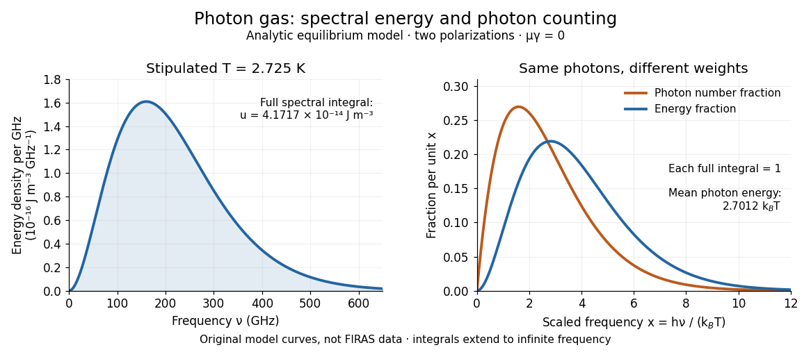
A motivating observation is the cosmic microwave background spectrum measured by the Far Infrared Absolute Spectrophotometer (FIRAS) aboard COBE. Its apparatus used a polarizing Michelson interferometer, with one input viewing a roughly seven-degree sky patch and the other an internal blackbody. Scanning mirrors changed the optical path length difference; heat-sensitive detectors recorded the varying power, and Fourier transform spectroscopy recovered the spectral difference. Operation outside the terrestrial atmosphere removed atmospheric emission and absorption, while shielding and cooling the optics in a helium cryostat suppressed the instrument's own radiation. ^[ref]

Absolute calibration came from moving an external blackbody into the sky aperture, filling the same beam used for the sky. This was an iron-loaded epoxy absorber shaped as a re-entrant cone. Repeated reflections made it a close approximation to a blackbody, while thermometers supplied its temperature. Mather and colleagues explicitly evaluated reflections, temperature gradients, radiation leaking through the material and leakage around its edge. These are limits on how faithfully the calibrator realizes thermal equilibrium radiation, rather than details that can be eliminated merely by calling it black. ^[ref]

During sky observations the internal blackbody temperature was adjusted to nearly null the spectral difference, reducing gain and drift errors. Fixsen and colleagues' 1996 analysis used calibrated spectra over wavenumbers $2$ to $21\mathrm{c}{\mathrm{m}}^{-1}$, about $60$ to $630\mathrm{GHz}$. They separated the sky's spatially uniform component, its dipole and Galactic emission, and varied sky cuts and foreground templates as controls. The resulting cosmic microwave background spectrum agreed with a single Planck function, with reported RMS deviations below 50 parts per million of its peak brightness. This is a residual statistic over the analyzed spectrum, not a pointwise relative error bound at every frequency. ^[ref]

The observation motivates using a photon gas as a physical model rather than merely a formal counting exercise. Its interpretation has a clear boundary: agreement with Planck's law constrains departures from an equilibrium spectral shape within the calibrated band and foreground assumptions; it does not directly measure radiation pressure or entropy density of a photon gas. Nor does it establish that today's cosmic microwave background is continually re-equilibrating with matter. A previously thermal spectrum can retain its Planck function shape as expansion of the universe lowers every photon frequency in the same proportion. The usefulness of the model is that one measured spectral temperature, together with its equilibrium assumptions, predicts energy density, radiation pressure, photon number density and entropy density of a photon gas consistently.

Planck's law gives the spectral radiance of an ideal blackbody in thermal equilibrium at absolute temperature $T>0$. It predicts how much power is carried in each small frequency or wavelength interval, per projected area and per solid angle. The whole curve is determined by $T$: no material-specific parameter enters this ideal Planck function.

Writing $\nu$ for frequency in hertz and $\lambda$ for wavelength in metres, the two forms of the Planck function areHere $h$ is the Planck constant, $k_B$ the Boltzmann constant, and $c$ the speed of light in vacuum. Their exact values in the International System of Units are $h=6.62607015\times 10^{-34}\mathrm{J}\mathrm{s}$, $k_B=1.380649\times 10^{-23}\mathrm{J}{\mathrm{K}}^{-1}$, and $c=299792458\mathrm{m}{\mathrm{s}}^{-1}$. ^[ref]

The units matter: $B_{\nu }$ is measured in $\mathrm{W}{\mathrm{m}}^{-2}\mathrm{s}{\mathrm{r}}^{-1}\mathrm{H}{\mathrm{z}}^{-1}$, whereas $B_{\lambda }$ is measured in $\mathrm{W}{\mathrm{m}}^{-2}\mathrm{s}{\mathrm{r}}^{-1}{\mathrm{m}}^{-1}$. Both are spectral radiance, rather than radiant exitance or energy density. To report $B_{\lambda }$ per micrometre, multiply its per-metre value by $10^{-6}$; a micrometre-wide interval is $10^{-6}$ metres wide.

For a computed example, at $T=6000\mathrm{K}$ and $\lambda =0.500\mu \mathrm{m}$, the exponent is $hc/(\lambda k_{B}T)\approx 4.79592$. Substitution into Planck's law gives $B_{\lambda }\approx 3.17569\times 10^{13}\mathrm{W}{\mathrm{m}}^{-2}\mathrm{s}{\mathrm{r}}^{-1}{\mathrm{m}}^{-1}$, or $3.17569\times 10^7\mathrm{W}{\mathrm{m}}^{-2}\mathrm{s}{\mathrm{r}}^{-1}$ per micrometre. At the same wavelength, the illustrative temperatures $3000\mathrm{K}$ and $4500\mathrm{K}$ give $2.60268\times 10^5$ and $6.37793\times 10^6$ in the latter units. These are ideal predictions for stipulated temperatures.

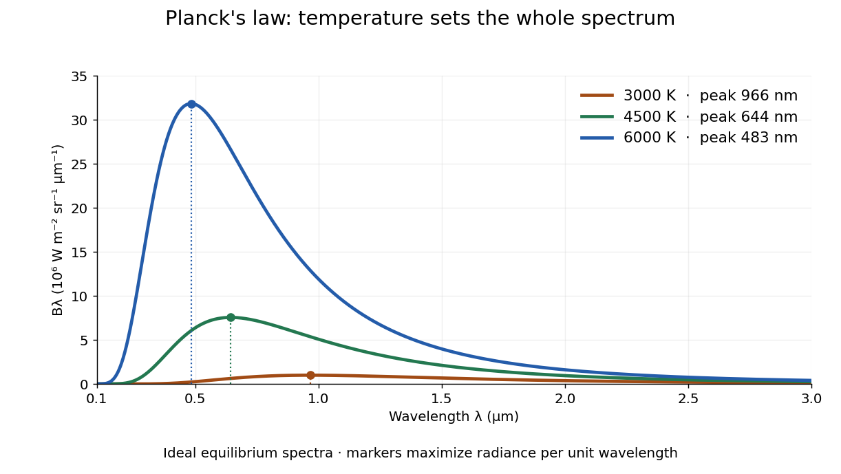
The key change of variables is $\nu =c/\lambda$. Corresponding positive intervals carry the same power, so $B_{\lambda }d\lambda =B_{\nu }|d\nu |$ andEqual-width wavelength intervals have unequal widths in frequency; the factor $c/{\lambda }^2$ compensates for this. Merely replacing the horizontal-axis labels of $B_{\nu }$ by $c/\nu$ does not produce $B_{\lambda }$. This explains the frequency and wavelength peaks of Planck's law.

A short derivation uses the Boltzmann distribution for a single electromagnetic mode with thermal energies $nh\nu$, $n=0,1,\dots$. Put $q=e^{-h\nu /(k_{B}T)}$. The geometric series gives $Z={\sum }_{n\ge 0}{q}^n=(1-q{)}^{-1}$ and mean thermal energy $h\nu q/(1-q)$. The electromagnetic mode density in a box, including both independent polarization of an electromagnetic wave states of a photon, is $8\pi {\nu }^2/c^3$ per volume per unit frequency. Multiplication gives spectral energy density $u_{\nu }=8\pi h{\nu }^3/[c^3(e^{h\nu /(k_{B}T)}-1)]$; isotropy gives $B_{\nu }=c{u}_{\nu }/(4\pi )$. This counts thermal excitation energy, excluding zero-point energy. ^[ref]

Planck's law connects quantum mechanics to a measurable radiation curve. Its small-$h\nu /(k_{B}T)$ limit is the Rayleigh-Jeans law, $B_{\nu }\approx 2k_{B}T{\nu }^2/c^2$; its large-$h\nu /(k_{B}T)$ limit is the Wien approximation, $B_{\nu }\approx (2h{\nu }^3/c^2)e^{-h\nu /(k_{B}T)}$. The suppression at high frequency makes the total energy density finite. Integrating the curve gives the Stefan–Boltzmann law, while locating its peak gives Wien's displacement law. Thus one formula predicts both the spectral shape and the total emission.