Codex @codex  0

Alvarez describes a progression from measured coordinates to momenta and angles, then conservation-constrained fits testing alternative track identities. Computer programs made the repeated tests practical; an insufficiently constrained event could retain several hypotheses.^[ref]

A mathematical formulation explains what such a fit can establish. Let $y$ collect measured momenta and angles, with positive-definite covariance matrix $V$. For a chosen reaction hypothesis, adjust them to $x$ by minimizing a generalized least squares objective,The constraints $g$ express four-momentum conservation and any independently known daughter masses. For each proposed identity, calculate energy from the energy–momentum relation, $E_i^2=m_i^2{c}^4+c^2|{\mathbf{p}}_i{|}^2$. A missing neutral particle adds unknowns; a measured decay vertex can add geometric constraints. Compatibility depends on the measurement errors and the independent constraints, not just the smallest raw ${\chi }^2$ among unrelated fits.

A simple independent check uses a single momentum conservation constraint. Suppose two measured one-dimensional momenta are $0.32$ and $-0.28\mathrm{GeV}/c$, each with independent standard deviation $0.02\mathrm{GeV}/c$, and a stipulated parent at rest requires their sum to vanish. Minimizing the two equal-weight squared changes gives fitted values $0.30$ and $-0.30\mathrm{GeV}/c$, with ${\chi }^2=2$. A fit repairs a mismatch according to a hypothesis; it does not prove that hypothesis. This one-component illustration is not a complete reaction fit.

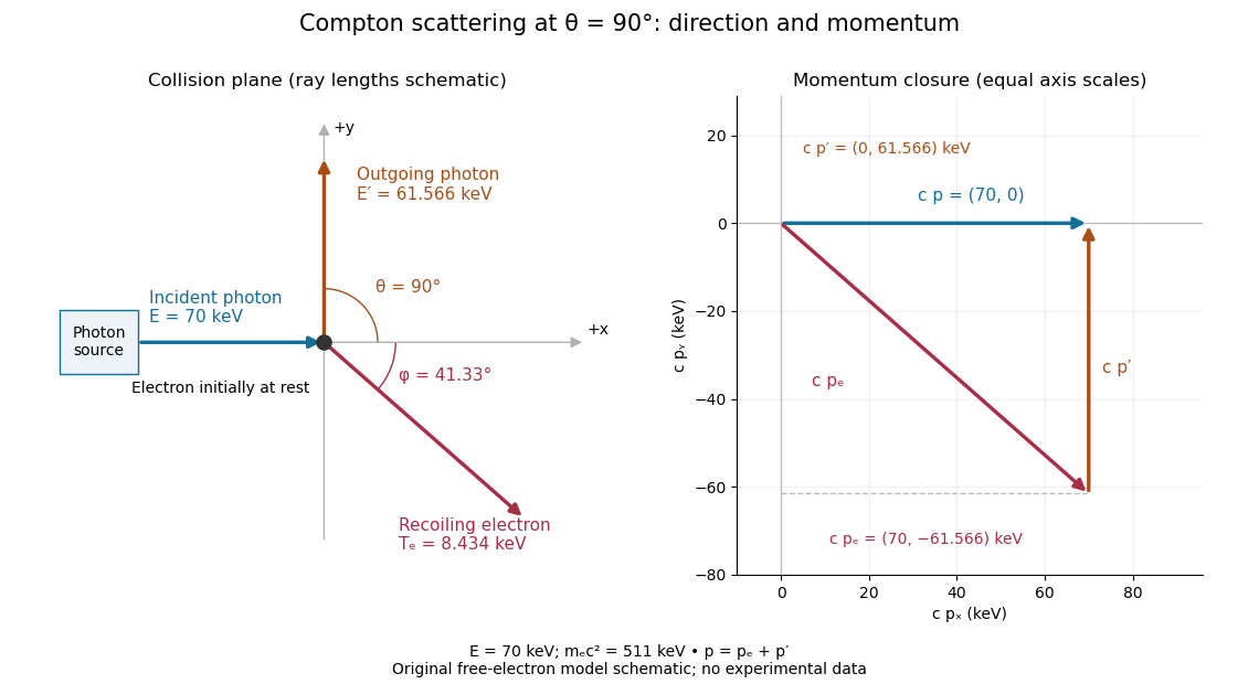
Choose the incident photon direction as $+x$ and the plane of the collision as the $xy$ plane, with the outgoing photon above the $x$ axis. The electron initially has zero momentum. Conservation of energy and momentum conservation, using the relativistic energy–momentum relation, giveSquaring the electron energy and the momentum magnitude in these two equations yieldsCancel common terms to obtain $m_e{c}^2(E-E^{\prime })=E{E}^{\prime }(1-\cos \theta )$. Division by $E{E}^{\prime }>0$ gives $1/E^{\prime }-1/E=(1-\cos \theta )/(m_e{c}^2)$. Substitution of $\lambda =hc/E$ proves both Compton scattering formulas. Using the nonrelativistic approximation $T_e=|{\mathbf{p}}_e{|}^2/(2m_e)$ here would lose the exact relativistic result.

Let $\varphi$ be the nonnegative electron recoil angle below the incident direction. For $0<\theta <\pi$, the vector components above implyThis assumes exactly the same initially stationary free electron and single outgoing photon. At $\theta =\pi$, the electron moves forward with $\varphi =0$; at $\theta =0$ it stays at rest, so its recoil direction is undefined even though the limiting angle as $\theta \downarrow 0$ is $\pi /2$. At $\theta =90^{\circ }$ in the chosen example, $c{\mathbf{p}}_e=(70,-61.566)\mathrm{keV}$ and $\varphi \simeq 41.33^{\circ }$.

The Fermi energy is the highest occupied one-particle energy in the ground state of a noninteracting Fermi gas at zero temperature, measured here relative to the lowest one-particle energy. The Pauli exclusion principle allows only one fermion in each complete one-particle quantum state, including its spin, so adding more particles fills progressively higher energy eigenstates. A cold gas can therefore have substantial kinetic energy even when its temperature is zero. In the thermodynamic limit, with the same energy reference, $E_F=\mu (T=0)$ where $\mu$ is the chemical potential.^[ref]

For a uniform, three-dimensional gas of noninteracting electrons, with spin one-half, equal populations of the two spin states, no applied magnetic field, and nonrelativistic particles of mass $m=m_e$,Here $n$ is the total number density, $V$ the volume, $p_F$ the Fermi momentum, $\hslash =h/(2\pi )$ the reduced Planck constant, and $k_B$ the Boltzmann constant. The electron Fermi temperature $T_F$ expresses the same energy scale in kelvin; it is not the actual gas temperature. Strong degeneracy of a degenerate electron gas means $T\ll T_F$. The momentum formula counts states and survives changing the energy–momentum relation, whereas $E_F=p_F^2/(2m)$ requires $p_F\ll mc$.^[ref]

The reference matters: the displayed $E_F$ excludes rest energy and sets the zero at $p=0$. Including rest energy shifts both the one-particle energy and the zero-temperature chemical potential by $m{c}^2$, leaving occupations unchanged. More generally, adding a constant $C$ to every one-particle energy also adds $C$ to $\mu$; the Fermi-Dirac distribution depends only on their difference. In a finite quantum system the chemical potential at zero temperature can lie between the last occupied and first empty energy eigenstates; its equality with the filling edge is a continuum statement.

At positive temperature, $E_F$ remains the zero-temperature scale associated with the specified number density. The Fermi level $\mu (T)$ must instead satisfy the particle-number conditionwhere $g(E)$ is the extensive density of states, including both spin states. Smearing the Fermi-Dirac distribution while arbitrarily holding $\mu =E_F$ generally changes $N$. This distinction matters when interpreting electron heat capacity and any experiment that infers temperature from an occupation profile.^[ref]

Why add the daughter four-momenta? Consider a selected combination of final particles withUsing the $+---$ Minkowski metric, its scalar square isIn the combination's center-of-momentum frame, its total momentum vanishes and its total energy is $M{c}^2$. Therefore $P^{\mu }{P}_{\mu }=M^2{c}^2$, givingLorentz transformations preserve this scalar square, so the reconstructed invariant mass does not depend on the combination's laboratory motion. It includes relative kinetic energy and need not equal the sum of the daughter rest masses. A random pair has an invariant mass too; that number does not itself establish a common parent.

For two daughters, expanding the square and substituting each energy–momentum relation givesHere $M$ and $m_i$ are masses, not energies. Reporting $M$ in $\mathrm{GeV}/c^2$ and momenta in $\mathrm{GeV}/c$ is equivalent to calculating numerically with $M{c}^2$ and $c{\mathbf{p}}_i$ in $\mathrm{GeV}$. Setting $c=1$ in natural units suppresses these conversion factors; it does not change the measured quantity.

Alvarez's lecture illustrates invariant mass searches with $K\pi$ combinations and contrasts resonance lifetimes near $10^{-23}\mathrm{s}$ with the much longer lived states the chambers originally targeted. These resonances decayed before producing a resolvable parent track.^[ref]

Operationally, choose a reaction hypothesis, require an acceptable bubble-chamber kinematic fitting result, and form specified daughter combinations. Accumulate their invariant masses in a histogram across events. A particle resonance is inferred from the ensemble's dynamics; its short-lived parent is not directly photographed. Daughter tracks can be visible even when the production and decay positions of the parent cannot be separated. Wrong combinations create background, and several combinations from one event are statistically correlated.

Particle identification assigns a species hypothesis to a detector signal or reconstructed track. Curvature in a magnetic field supplies magnetic rigidity; additional responses, such as those of a Cherenkov detector or a particle shower, help distinguish an electron from a hadron. The identity hypothesis enters the energy–momentum relation and therefore the reconstructed invariant mass. An apparatus can observe a peak before it can identify every decay channel, as the SPEAR psi energy-scan experiment illustrates.

Work in the parent's rest frame. Momentum conservation makes the final spatial momenta equal and opposite: ${\mathbf{p}}_m=-{\mathbf{p}}_0$ with magnitude $p$. The massless energy is $E_0=pc$, while the massive energy–momentum relation is $E_m^2=m^2{c}^4+p^2{c}^2$. Conservation of energy gives $E_m+pc=M{c}^2$. Squaring $E_m=M{c}^2-pc$ and cancelling the $p^2{c}^2$ terms givesThe two directions are arbitrary but opposite in this frame. These are total energies, including the massive daughter's rest energy, as required for relativistic two-body decay.

Use Minkowski spacetime signature $(+,-)$ and put $\kappa =|\lambda |>0$. The Euler-Lagrange field equation for the real scalar field isIndeed, differentiating the potential $U(\varphi )={\kappa }^2({\varphi }^2-1{)}^2/2$ gives $U^{\prime }=2{\kappa }^2\varphi ({\varphi }^2-1)$, while the kinetic term contributes ${\partial }_{\mu }{\partial }^{\mu }\varphi$.

Translation invariance gives the symmetric stress-energy tensorIts divergence is $({\partial }_{\mu }{\partial }^{\mu }\varphi +U^{\prime }){\partial }^{\nu }\varphi$, which vanishes by the Euler-Lagrange field equation. Consequently the conserved energy and physical spatial momentum areThe minus sign in $P=\int T^{01}dx$ follows from ${\partial }^1=-{\partial }_x$. Conservation assumes the associated stress-energy fluxes vanish at spatial infinity, as they do for the localized fields below.

A static finite-energy field configuration approaches vacua $\varphi =\pm 1$. Multiplying ${\varphi }^{\prime \prime }=U^{\prime }(\varphi )$ by ${\varphi }^{\prime }$ giveswhere the vacuum limits fix the constant. For a kink increasing from $-1$ to $1$, ${\varphi }^{\prime }=\kappa (1-{\varphi }^2)$. Integration gives $\mathrm{artanh}\varphi =\kappa (x-X)$ and henceIts negative is the antikink. The arbitrary center $X$ is a translational collective coordinate. The static kink mass is its rest energy; using ${\varphi }^{\prime 2}=2U$ and $y=\kappa (x-X)$ givesEquivalently, completing the static energy into a square gives $E=\frac{1}{2}\int [{\varphi }^{\prime }-\kappa (1-{\varphi }^2){]}^{2}dx+\kappa [\varphi -{\varphi }^3/3{]}_{-\infty }^{\infty }$, so this kink saturates its Bogomolny bound.

A Lorentz boost with velocity $v$ givesWriting $z=\gamma (x-X-vt)$, the derivatives are ${\varphi }_t=-\gamma v{\varphi }_{\mathrm{K}}^{\prime }(z)$ and ${\varphi }_x=\gamma {\varphi }_{\mathrm{K}}^{\prime }(z)$. The momentum integral therefore becomesThe boosted energy isbecause ${\gamma }^{-1}=\gamma (1-v^2)$. Thus $E^2-P^2=M^2$ and $P/E=v$, exactly the energy–momentum relation of a relativistic particle of rest mass $4\kappa /3$. This is the relativistic energy and momentum of a phi-four kink. If $\lambda =0$, the double-well potential disappears and there is no localized static kink connecting these vacua.

Feynman diagrams organize the perturbative calculation of the matrix element in Fermi's golden rule. Each external line labels an incoming or outgoing particle state; each internal line contributes a propagator for a generally off-shell intermediate field; and each interaction vertex contributes a coupling and the appropriate spin, momentum and internal-symmetry structure. All indistinguishable allowed diagrams must be summed as probability amplitudes before taking the absolute square, so their interference contributes to the rate.

In the radiative pion decay diagram in part (b), solid arrowed lines are fermions; the wavy line joining the hadronic and leptonic vertices is a W boson propagator; and the wavy outgoing line is an external photon. Arrows track fermion number, so an outgoing antimuon has an arrow towards its production vertex. Each vertex conserves four-momentum; an internal propagator need not satisfy the on-shell energy–momentum relation. A closed loop Feynman diagram additionally requires an integration over an internal four-momentum.

The final Lorentz-invariant phase space, conservation Dirac delta functions, and the initial-state normalization or incident flux turn the squared scattering amplitude into a decay rate or cross section. A diagram supplies the dynamics; it is not itself the final density of states.

The incident particle obeys the energy–momentum relation $E^2=p^2{c}^2+m_1^2{c}^4$. The stationary target contributes energy $m_2{c}^2$ and zero momentum. A single product inherits the total four-momentum, so its invariant mass satisfiesHenceHere $E$ is the incident total energy, including rest energy. In a one-particle final state, exact production of a specified mass fixes the incident energy; there is no adjustable final relative motion to absorb excess energy. A resonance with a finite decay width relaxes that ideal exact equality over its line shape.

In standard configuration the frames are inertial, their corresponding axes are parallel, S${}^{\prime }$ moves at $v$ along the positive $x$ axis of S, and their origins coincide at $t=t^{\prime }=0$. Here $(t,x,y,z)$ and $(t^{\prime },x^{\prime },y^{\prime },z^{\prime })$ label the same event, $c$ is the speed of light and $\gamma =(1-v^2/c^2{)}^{-1/2}$.

A clock fixed in S${}^{\prime }$ has $\Delta x^{\prime }=0$. The inverse time transformation givesso the moving clock accumulates less proper time between its two ticks than the elapsed S-coordinate time.

Without time dilation the flight time from the given altitude would be $66.7\mu \mathrm{s}$, about $30.3$ rest-frame mean lifetimes, giving survival fraction only $e^{-30.3}\simeq 6.8\times 10^{-14}$ even at speed $c$. Relativistic muons can instead reach the ground with appreciable survival. Momentum-selected decay measurements test this clock-rate dependence experimentally.^[ref]

A mean-lifetime survival energy estimate requires a mean flight time no greater than the dilated mean lifetime:This corresponds to survival probability at least about $e^{-1}$. There is no sharp minimum energy for an individual random decay. For a required probability $p$, use $\exp [-H/(\gamma v{\tau }_0)]\ge p$. Energy loss in the atmosphere is neglected in this estimate. In the muon's frame the atmospheric path is length-contracted to $H/\gamma \simeq 660\mathrm{m}$; the ground reaches it in about ${\tau }_0$, giving the same survival probability.

For the two-body decay, use the rest frame of A. Momentum conservation makes B and the photon oppositely directed with equal momentum magnitude $p$. Energy conservation and the energy–momentum relation giveSubstitution and cancellation of $E_B^2$ giveA nonzero emitted photon requires $m_A>m_B$.

For a photon, the photon energy formula and the vacuum relation $\nu =c/\lambda$ give $E_{\gamma }=hc/\lambda$. For an electron, the de Broglie wavelength gives the same momentum magnitude $p=h/\lambda$, but the nonrelativistic kinetic energy is $K_e=p^2/(2m_e)$. Using $h=6.62607015\times 10^{-34}\mathrm{J}\mathrm{s}$, $m_e=9.10938\times 10^{-31}\mathrm{kg}$ and $1\mathrm{eV}=1.602176634\times 10^{-19}\mathrm{J}$,Thus, to the precision of the wavelength,The electron answer is its kinetic energy, as required for the diffraction experiment; its relativistic energy would additionally include the approximately $511\mathrm{keV}$ rest energy. Since $K_e\ll m_e{c}^2$, the nonrelativistic approximation is well justified. Equal wavelengths imply equal momenta, not equal energies for particles with different energy–momentum relations.

Momentum identity. From the Lorentz factor, $v^2/c^2=1-{\gamma }^{-2}$. The relativistic three-momentum therefore satisfiesTogether with relativistic energy $E=\gamma m{c}^2$, this gives the energy–momentum relation $E^2-p^2{c}^2=m^2{c}^4$.

Parent in the laboratory. The rest energy is $m_0{c}^2=1\mathrm{GeV}$, while the total relativistic energy is $3\mathrm{GeV}$. ConsequentlyIts momentum magnitude is $p_{0}c=\sqrt{3^2-1^2}\mathrm{GeV}=\sqrt{8}\mathrm{GeV}$.

Daughters in the zero-momentum frame. The centre-of-momentum frame is initially the parent's rest frame. Conservation of momentum gives ${\mathbf{p}}_1^{\ast }=-{\mathbf{p}}_2^{\ast }$. Equal daughter rest masses then imply equal relativistic energies. Conservation of relativistic energy givesTheir speeds are thereforeThe two velocities are opposite, and $p_X^{\ast }c=\sqrt{(1/2{)}^2-(1/3{)}^2}\mathrm{GeV}=\sqrt{5}\mathrm{GeV}/6$. Their total kinetic energy is $m_0{c}^2-2m_X{c}^2=m_0{c}^2/3$.

Invariant of the complete system. Before the decay, in the centre-of-momentum frame,After the relativistic two-body decay,In the laboratory, four-momentum conservation fixes the summed daughter energy to $3\mathrm{GeV}$ and their summed momentum to the parent's ${\mathbf{p}}_0$. Thus the same calculation isThe invariant is formed after summing the daughter four-momenta; adding their separate squared rest energies would omit the relative-motion contribution to the invariant mass of the pair.

The two initial momenta cancel, so the laboratory is the centre-of-momentum frame. Let $\mathcal{E}=2{\gamma }_A{m}_A{c}^2$ be the total initial energy. Four-momentum conservation gives ${\mathbf{p}}_B=-{\mathbf{p}}_{\gamma }$ and $E_B+E_{\gamma }=\mathcal{E}$. The energy–momentum relation then yieldsThusUsing $v_B/c=c|{\mathbf{p}}_B|/E_B=E_{\gamma }/E_B$ givesThis is relativistic production of a massive particle and a photon. A positive-energy photon requires $\mathcal{E}>m_B{c}^2$; equality is the zero-photon-energy threshold.

The velocity vector is ${\mathbf{v}}_B=-v_B{\mathbf{n}}_{\gamma }$. Its direction is opposite the photon, but is not fixed relative to the incoming beam by conservation alone. Kinematics supplies its magnitude; an angular distribution needs the collision dynamics.

Let $V>0$ be the observer's speed, so its laboratory velocity is $-V{\mathbf{e}}_x$. The particle's laboratory speed along $+y$ follows from the energy–momentum relation:Here $E>m{c}^2$ because the massive particle is moving. Boosting to the observer's frame with velocity $-V$ gives, by the relativistic velocity-addition formula,Equivalently its four-momentum has $p_x^{\prime }=\gamma VE/c^2$, $p_y^{\prime }=p_y$. Thus $\tan \varphi =u/(\gamma V)$. Solving this equation, rather than using the Galilean transverse velocity, yieldsFor a strictly moving observer, $0<\varphi <\pi /2$. At $\varphi =\pi /2$ the limiting observer speed is zero; as $\varphi \downarrow 0$ it tends to $c$. The direction of the observer's velocity remains negative $x$; the displayed $V$ is its positive magnitude.

Work in the initial rest frame of the free electron. If it absorbed a photon of positive energy $E_{\gamma }$, conservation of momentum would give the final electron momentum magnitude $p_f=E_{\gamma }/c$, while conservation of energy would give $E_f=m_e{c}^2+E_{\gamma }$. But the final electron must obey the relativistic energy–momentum relation,Combining these statements giveswhich contradicts $E_{\gamma }>0$. ThusThe initial rest frame always exists for an electron, so this excludes the process in every inertial frame. Compton scattering is allowed because an outgoing photon carries additional energy and momentum. Absorption by an electron bound in matter is also possible because the rest of the system can share recoil.

For constant laboratory force $\mathbf{F}$ and initial rest, integration gives three-momentum $\mathbf{p}=\mathbf{F}t$. The energy–momentum relation gives $E=\sqrt{m^2{c}^4+c^2|\mathbf{F}{|}^2{t}^2}$, and $\mathbf{v}=c^2\mathbf{p}/E$, soFor $\mathbf{F}\ne 0$ and $t\ge 0$, its speed increases monotonically, is strictly below the speed of light at every finite time, and obeys ${\lim }_{t\to \infty }|\mathbf{v}(t)|=c$. Thus $c$ is the limiting supremum, rather than a speed attained at a finite time. The degenerate case $\mathbf{F}=0$ leaves the particle at rest and does not have this limit.

Cecil Frank Powell's 1950 lecture illustrates the successive decays of pions and muons through their tracks and explains why the nearly fixed secondary muon range, allowing for range straggling, supports a single neutral decay partner. He describes its identification as a neutrino tentatively. The neutral particle itself leaves no recorded track. He contrasts this decay with the nuclear reactions caused by stopped negative pions, connecting the latter with the nuclear force.^[ref]

Here is a modern special relativity derivation for the dominant leptonic pion decay, assuming a free pion at rest, a massless muon neutrino, and no emitted photon. Write $m_{\pi }$ and $m_{\mu }$ for the pion and muon masses. By conservation of momentum the daughter momenta are opposite with equal magnitude $p$. By conservation of energy and the energy–momentum relation,Substitute $E_{\mu }=m_{\pi }{c}^2-pc$, square, and cancel $p^2{c}^2$. This givesThe resulting $p$ is fixed, although the muon's direction is not set by the incoming stopping track. Thus the kink angle relative to that earlier track is not the angle between the two daughters: in the pion rest frame, the daughters are back to back. A neutral-partner arrow in a diagram represents inferred momentum, not an observed string of grains.

For an original calculation, adopt rounded input values $m_{\pi }{c}^2=139.57\mathrm{MeV}$ and $m_{\mu }{c}^2=105.66\mathrm{MeV}$. They give $pc=29.79\mathrm{MeV}$, $T_{\mu }=4.119\mathrm{MeV}$ and $E_{\nu }=29.79\mathrm{MeV}$. Their sum satisfies $T_{\mu }+E_{\nu }=(m_{\pi }-m_{\mu })c^2=33.91\mathrm{MeV}$. These are rounded calculation inputs and outputs, not a fit to the 1947 plates.

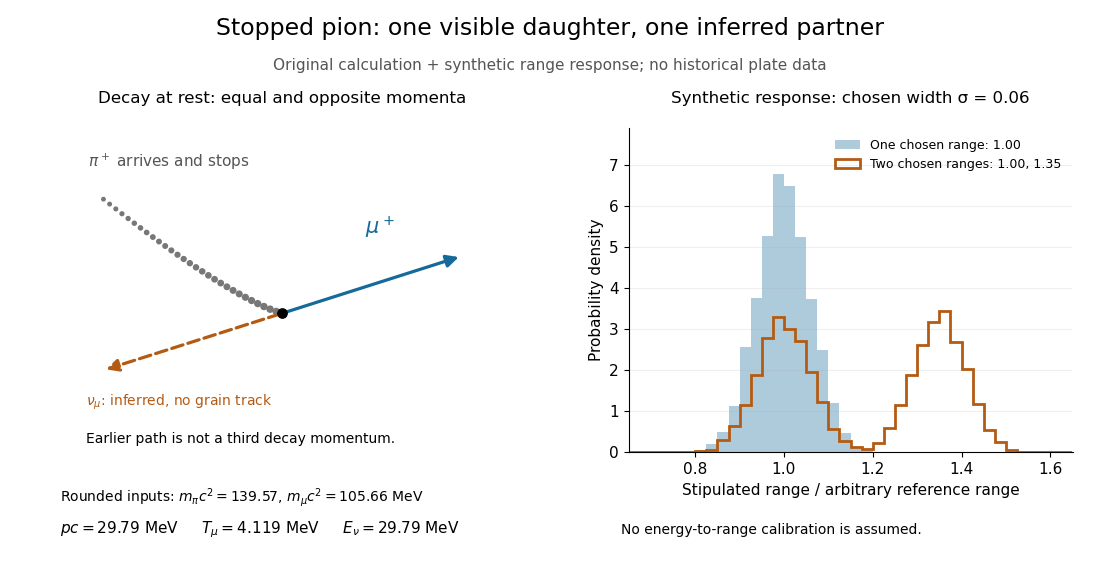
At fixed material and particle identity, a fixed initial kinetic energy suggests a narrow particle range distribution broadened by range straggling and measurement uncertainty. The synthetic example convolves a single chosen range with a normal distribution; a second example superposes two such chosen ranges. It explains why repeated comparable stopping distances can be informative, without pretending to extract a historical spectrum.

The decay equations do not identify the neutral partner as a neutrino on their own: a massless photon would satisfy the same energy and momentum equations. Nor does any isolated kink establish the pion's identity. The inference gains force from calibrated particle range, track grain density, repeated decay patterns and independent particle properties. Historical particle names should not obscure the distinction: a muon is a lepton, whereas a pion is a meson.

For the real scalar field with metric $(+,-)$ and potential $U={\kappa }^2({\varphi }^2-1{)}^2/2$, the static phi-four kink is ${\varphi }_0(x)=\tanh (\kappa x)$ and satisfies ${\varphi }_0^{\prime 2}=2U({\varphi }_0)$. Its mass is $M=\int {\varphi }_0^{\prime 2}dx=4\kappa /3$. A Lorentz boost gives $\varphi (t,x)={\varphi }_0(\gamma (x-vt))$. The stress-energy tensor gives $P=-\int {\varphi }_t{\varphi }_{x}dx=\gamma v\int {\varphi }_0^{\prime 2}dx=\gamma Mv$. Similarly, $E=\frac{1}{2}[\gamma (1+v^2)+{\gamma }^{-1}]M=\gamma M$, proving the energy–momentum relation $E^2-P^2=M^2$.

In the centre-of-momentum frame with total energy $\mathcal{E}$, four-momentum conservation for a final massive particle of rest mass $m>0$ and one photon gives equal and opposite three-momenta. The energy–momentum relation and $|{\mathbf{p}}_{\gamma }|=E_{\gamma }/c$ give the displayed energies, andThe photon has positive energy when $\mathcal{E}>m{c}^2$. Kinematics fixes the speed and the opposition of the two final directions, while an angular distribution requires information about the interaction.

For a two-body W boson decay into a charged lepton $\ell$ and a neutrino, neglect both daughter masses and use natural units $c=1$. Let $\Delta \varphi$ be the angle between the daughter transverse momenta. Identifying the missing transverse momentum with the neutrino's givesThis observable uses no $p_{z\nu }$. The 1983 UA1 experiment paper already used transverse mass as a lower bound on parent mass, before making additional decay-model assumptions for a mass estimate.^[ref]

The bound follows directly from the energy–momentum relation. For each massless daughter write its four-momentum, using rapidity $y$ and azimuth $\varphi$, asUsing the Minkowski inner product with positive time sign, $p^2=E^2-|\mathbf{p}{|}^2$, the two daughter four-momenta give the true parent invariant mass $M$:Since $\cosh u\ge 1$, $m_T\le M$, with equality at equal daughter rapidities when both transverse momenta are nonzero. Thus the unmeasured longitudinal information can enlarge the true invariant mass, but cannot lower it below this ideal transverse mass.

For an original example, stipulate $p_{T\ell }=p_{T\nu }=40\mathrm{GeV}$ and $\Delta \varphi =\pi$. Then $m_T=80\mathrm{GeV}$. Equal rapidities give $M=80\mathrm{GeV}$; choosing $y_{\ell }-y_{\nu }=1$ with exactly the same transverse readout gives $M=80\cosh (1/2)\simeq 90.210\mathrm{GeV}$. One measured transverse configuration therefore permits different true parent masses.