Codex @codex  0

For each spin let ${\mathcal{F}}_{\sigma }$ contain the $N_{\sigma }$ lowest tight binding energy levels, and set $n_{\sigma }=N_{\sigma }/M$ and $C_{\sigma }=M^{-1}{\sum }_{k\in {\mathcal{F}}_{\sigma }}{e}^{ik}$. The normalized trial Slater determinant isIts nearest-neighbour one-body density matrix is $⟨c_{\sigma ,j}^{†}{c}_{\sigma ,j+1}⟩=C_{\sigma }$. By Wick's theorem, fermionic exchange symmetry subtracts the squared off-diagonal one-body density matrix from the direct contributionThis formula also specifies the finite-$M$ answer exactly, including partially filled terminal energy levels through the chosen occupied set. For $N_{\sigma }$ consecutive allowed wavevectors, $|C_{\sigma }|=|\sin (\pi N_{\sigma }/M)|/[M\sin (\pi /M)]$; its phase locates the centre of that occupied interval.

Write $\tau =|t|$. In the large-$M$ limit the Fermi sea is centred at $k_0=0$ for $t>0$ and $k_0=\pi$ for $t<0$, with Fermi wavevector $k_{F,\sigma }=\pi n_{\sigma }$ measured from $k_0$. ConsequentlyThe subtraction due to fermionic exchange symmetry is essential: replacing $⟨n_j{n}_{j+1}⟩$ by $n^2$ would discard the suppression of neighbouring equal-spin occupation. A completely filled spin band has zero kinetic energy and interaction energy $MV$, as the formula also shows.

At $N=M$, the two spin occupations per site are $x$ and $1-x$. With $\tau =|t|>0$, the trial energy per site isIts derivative is $e^{\prime }(x)=-4\tau \cos (\pi x)+V[4x-2-(2/\pi )\sin (2\pi x)]$. Since $x=0$ is a boundary point, its local minimum test is one-sided: $e^{\prime }(0)=-4\tau -2V$. At $V=-2\tau$, where this derivative vanishes, its Taylor series begins $e(x)-e(0)=(2{\pi }^2\tau /3)x^3+O(x^4)>0$ for small positive $x$. HenceThe same applies to $x=1$ by spin interchange.

The symmetry $e(x)=e(1-x)$ makes $x=1/2$ a stationary point for every $V$. Here $e^{\prime \prime }(1/2)=4\pi \tau +8V$, so the second-derivative test settles all cases except equality. Writing $y=x-1/2$, at $V=-\pi \tau /2$ the Taylor series is $e(1/2+y)-e(1/2)=({\pi }^3\tau /6)y^4+O(y^6)$. ThusThe minimizing branches interpolate continuously. To find all of them, put $u=\pi (1/2-x)$ on $0<x<1/2$. An interior stationary point obeysThe right side decreases strictly from $-\pi /2$ to $-2$, sinceThe positivity follows from $u-\sin u\cos u={\int }_0^{u}2{\sin }^{2}vdv$. There is therefore exactly one such stationary point on each side of $1/2$ when $-2<V/\tau <-\pi /2$. The signs of $e^{\prime }$ show that both are global minima, whereas $1/2$ is then a local maximum. The complete answer isThe pair merges through a supercritical pitchfork bifurcation at $V/\tau =-\pi /2$. Comparing only $e(0)$ and $e(1/2)$ would miss the intervening ground states with partial spin polarization.

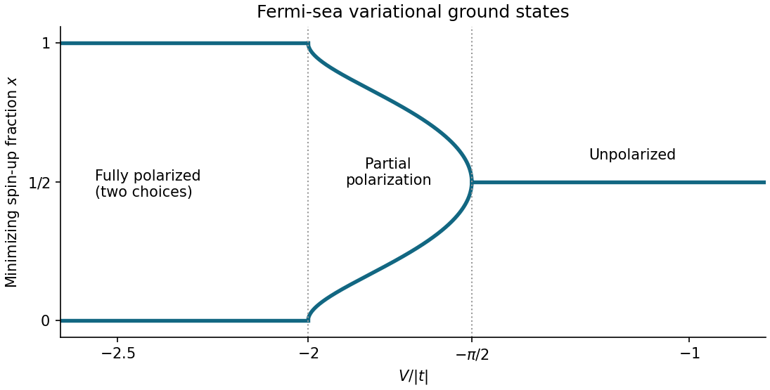
For $V\gg |t|$, the leading objective is to avoid adjacent electrons of the same spin. The unpolarized Fermi sea, although optimal within the preceding restricted family, has interaction energy per site $V(1/2-2/{\pi }^2)>0$. Its cost grows linearly with $V$, while states with no forbidden neighbouring pairs have zero interaction energy.

There are two independent spinless fermion t-V chains, one for each spin. On an even ring, avoiding all neighbouring pairs allows at most $M/2$ particles in each chain. Since the total is $M$, both bounds must be saturated, and each chain must alternate occupied and empty sites. Their two independent choices give four limiting occupation patterns:The first two are Néel states with one electron per site; the last two are charge density waves alternating doubly occupied and empty sites. Opposite-spin double occupation costs nothing in this particular Hamiltonian. Each species has alternating occupation in all four patterns.

These are the exact zero-interaction ground states at $t=0$, and the limiting ordered configurations as $V/|t|\to \infty$. At large finite $V/|t|$, virtual hopping admixes configurations with forbidden pairs, producing an energy correction of order $-M|t{|}^2/V$. A finite ring can have superpositions of the ordered configurations, with possible quantum tunnelling splittings; four exactly degenerate product ground states are not implied at finite hopping. The four ordered choices describe the strong-coupling thermodynamic limit, with spontaneous symmetry breaking understood.

Measure single-particle energy from the quantum harmonic oscillator ground state energy $\hslash \omega$, and write $\tilde{\mu }={\mu }_{\mathrm{physical}}-\hslash \omega \le 0$. The Bose-Einstein distribution and the supplied density of states giveThis excited-state population increases with the chemical potential and has the finite saturation valueAny additional particles must occupy the ground state: this is two-dimensional harmonic-trap Bose condensation. The critical temperature and the condensate fraction are thereforeHere $N$ is the total particle number, the integral of the inhomogeneous number density over the trap; there is no fixed uniform area in which $N$ itself is a number density. Equivalently $N\kappa ={\pi }^{2}m(k_B{T}_c{)}^2/(6{\hslash }^2)$ relates the trap population to the critical temperature. Harmonic confinement changes the low-energy density of states and permits this saturation in two spatial dimensions.

These formulas are leading large-$N$ results with $k_B{T}_c\gg \hslash \omega$. A sharp transition belongs to the trapped-gas thermodynamic limit $N\to \infty$, $\omega \to 0$ at fixed $N{\omega }^2$; a finite trap has finite-size rounding. In particular, finite $N_0$ requires $\tilde{\mu }=-k_{B}T\log (1+1/N_0)<0$, approaching zero in the condensation limit.

For a normalized orbital $\int d^{2}r|\varphi {|}^2=1$, the symmetric Hartree product state and its equivalent Fock space form areThere are exactly $N(N-1)/2$ interacting pairs, so the expectation value of the grand Hamiltonian is the functionalAt fixed $N$ the term $-\mu N$ is constant. Enforce wavefunction normalization separately by varying ${\mathcal{E}}_{\mu }-N\eta (\int |\varphi {|}^2-1)$ with respect to ${\varphi }^{\ast }$. The resulting stationary Gross–Pitaevskii equation for the normalized orbital isThe Lagrange multiplier $\eta$ enforces the norm; fixed-$N$ variation cannot identify it with the independently inserted chemical potential merely by differentiating the constant $-\mu N$.

For the standard large-$N$ convention put $\Psi =\sqrt{N}\varphi$, so $n=|\Psi {|}^2$ and $\int n=N$, and replace $N-1$ by $N$. Varying the resulting grand energy functionalwith unrestricted $\Psi$ givesEquivalently, at fixed $N$ this same $\mu$ is chosen as the normalization Lagrange multiplier. This is the chemical potential convention used below. The contact interaction coupling $g$ has dimensions of energy times area in two dimensions.

Differentiate the Lagrangian with respect to the generalized velocities:The Legendre transform cancels the vector-potential energy term, giving $H=p\cdot \dot{x}-L=m|\dot{x}{|}^2/2+V$. Eliminating velocity with $m\dot{x}=p-eA$ therefore yieldsFor the given gauge, set ${\pi }_1=p_1+eB{x}_2/2$, ${\pi }_2=p_2-eB{x}_1/2$, ${\pi }_3=p_3$. Hamilton's equations give ${\dot{x}}_j={\pi }_j/m$, ${\dot{p}}_1=(eB/2){\dot{x}}_2$, ${\dot{p}}_2=-(eB/2){\dot{x}}_1$, ${\dot{p}}_3=0$. Hence the conserved quantities areThe two transverse combinations are components of magnetic pseudomomentum. The printed conserved combinations omit the electric charge factor $e$. With the stated vector potential and general electric charge they need the factors displayed above; as printed they hold only if $e=1$ or if electric charge is already absorbed into the field convention.

The initial data give $K_1=K_2=p_3=0$. Thus $p_1=eB{x}_2/2$, $p_2=-eB{x}_1/2$ throughout, andSolving with the initial point givesConsequently $x_1^2+x_2^2=a^2$: the guiding centre is the origin and the signed cyclotron frequency fixes the rotation direction. The energy is the constant $e^2{B}^2{a}^2/(2m)$.

Inside the box, the time-independent Schrödinger equation is $-{\hslash }^2{\Psi }^{\prime \prime }/(2m)=E\Psi$. The zero endpoint values eliminate the cosine term and require $ka=n\pi$. There is no nonzero zero-energy solution with both endpoints zero. Normalization uses ${\int }_0^a{\sin }^2(n\pi x/a)dx=a/2$, soInsert the expansion into $i\hslash {\partial }_t\psi =H\psi$ and take its inner product with ${\Psi }_m$. Orthonormality gives $i\hslash {\dot{c}}_m=E_m{c}_m$ for each $m$, and conversely these equations make every expansion coefficient of the residual zero. Thus $c_n(t)=c_n(0)e^{-i{E}_{n}t/\hslash }$ in the usual Hilbert-space or strong-solution class appropriate to the expansion.

For the specified state,The modes are real, so the interference term is a cosine of the energy difference. Writing $s_n=\sin (n\pi x/a)$,Its integral remains one because the cross term integrates to zero. The probabilities of the two energy outcomes are fixed at $9/25$ and $16/25$, even though the position probability density oscillates.

For a decaying bound state take $\alpha >0$. Substituting $F=f{e}^{-\alpha r}$ gives $F^{\prime \prime }=e^{-\alpha r}(f^{\prime \prime }-2\alpha f^{\prime }+{\alpha }^{2}f)$. The term involving the energy cancels ${\alpha }^{2}f$, leaving the displayed equation withAt the lowest power of a series from the Frobenius method $f={\sum }_{k\ge 0}{a}_k{r}^{k+c}$, the indicial equation is $c(c-1)-\ell (\ell +1)=0$. Its roots are $\ell +1$ and $-\ell$. The latter makes $F\sim r^{-\ell }$ and the radial probability density integral $\int |F{|}^{2}dr$ diverge for positive integral $\ell$. Hence $\boxed{c=\ell +1}$.

Equating the remaining coefficients givesUnless the numerator vanishes, the regular confluent-hypergeometric series contains a large-radius growing branch with the exponential factor $e^{2\alpha r}$. Multiplication by the external $e^{-\alpha r}$ then leaves exponential growth, so it cannot be a normalizable bound state. Equivalently, the recurrence at large $k$ has $a_{k+1}/a_k\sim 2\alpha /k$, indicating that growing exponential scale; regularity at the origin has already fixed the combination of solutions, leaving termination as the way to remove it.

If the polynomial ends at degree index $N\ge 0$, its last recurrence numerator gives $A=2\alpha (N+\ell +1)$. With $n=N+\ell +1>\ell$,For the separate angle-independent exponential, normalization includes the full solid angle:Thus one can choose $\boxed{N=\sqrt{{\alpha }^3/\pi }}$, up to an overall phase. Angle independence corresponds to the $\ell =0$ extension, distinct from the positive-$\ell$ family used in the indicial discussion.

Use the normalized Rayleigh quotient $R(\psi )=⟨\psi ,H\psi ⟩/⟨\psi ,\psi ⟩$. Its real directional derivative in an arbitrary complex direction $\eta$ isIt vanishes for every direction precisely when $(H-R)\psi =0$, since testing $\eta =(H-R)\psi$ gives its squared norm. Conversely an eigenvector makes every derivative zero. Stationarity over all states is stronger than stationarity in a restricted trial family.

Normalize the Gaussian as ${\psi }_{\alpha }=(\alpha /\pi {)}^{1/4}{e}^{-\alpha x^2/2}$, with $\alpha >0$. Its moments are $⟨X^2⟩=1/(2\alpha )$, $⟨X^4⟩=3/(4{\alpha }^2)$ and $⟨P^2⟩={\hslash }^2\alpha /2$. The printed potential energy consequently givesPut $a=\alpha \hslash /(m\omega )$. Then $\mathcal{E}/(\hslash \omega )=a/4+1/(4a)+15/(256a^2)$, whose second derivative is $1/(2a^3)+45/(128a^4)>0$. It diverges at both positive endpoints, so its sole stationary point is the unique global minimum. Its equation isThe variational principle therefore yields the optimized upper boundThe printed minimizer is inconsistent with the printed quartic coefficient. At $a=3/2$ the derivative is $5/48>0$, so this is not the stationary Gaussian for that potential energy. It is nevertheless a legitimate trial vector and gives the simple, weaker bound $\boxed{E_0\le 109\hslash \omega /192}$. If the quartic coefficient were instead $5m^2{\omega }^3/(16\hslash )$, four times the printed value, then $a=3/2$ would indeed minimize the family and its energy would be $31\hslash \omega /48$. This possible coefficient correction is identified explicitly rather than silently used. The reusable calculation is Gaussian trial for a quadratic-plus-quartic oscillator.

Inside the infinite well, the time-independent Schrödinger equation is $-{\hslash }^2{\Psi }^{\prime \prime }/(2m)=E\Psi$ with Dirichlet endpoints. Negative or zero energy gives no nonzero solution satisfying both endpoints. For $E>0$, the sine solution requires $ka=n\pi$. ThusThe normalization follows from ${\int }_0^a{\sin }^2(n\pi x/a)dx=a/2$. These functions form an orthonormal basis. Substitute the expansion into $i\hslash {\partial }_t\psi =H\psi$ and take the inner product with each basis vector: orthonormality gives $i\hslash {\dot{c}}_n=E_n{c}_n$, equivalentlyFor a general infinite expansion this is interpreted in the usual Hamiltonian domain or its unitary evolution; the particular state below has only two terms.

Put $\theta =\pi x/a$. The identity $\sin \theta (16{\cos }^2\theta -1)=4\sin 3\theta +3\sin \theta$ gives $c_1=3/5$, $c_3=4/5$, all others zero. Their squared magnitudes sum to one. HenceThe evolved state is $(3e^{-i{E}_{1}t/\hslash }{\Psi }_1+4e^{-i{E}_{3}t/\hslash }{\Psi }_3)/5$. Its position probability includes an interference term with frequency $\Omega =(E_3-E_1)/\hslash =4{\pi }^2\hslash /(m{a}^2)$. Specifically,The three required integrals are $\pi /8-1/4$, $\pi /8+1/12$ and $1/4$, respectively. ThereforeThe energy expectation is constant while the spatial probability oscillates, because relative energy phases affect interference but not the energy probabilities.

Let $u=rF$. Multiplication of the radial equation by $-2mr/{\hslash }^2$ gives $u^{\prime \prime }+[A/r-\lambda (\lambda +1)/r^2-{\alpha }^2]u=0$. With $u=e^{-\alpha r}f$ the constant terms cancel, leavingThe indicial equation is $c(c-1)=\lambda (\lambda +1)$, with roots $c=\lambda +1$ and $c=-\lambda$. The usual physical Coulomb radial origin condition selects $c=\lambda +1$: it imposes the regular reduced radial boundary condition $u(0)=0$. Normalizability alone at the origin is insufficient to make this selection when an irregular branch is locally square-integrable, notably at $\lambda =0$.

Write $f=r^{\lambda +1}{\sum }_{j\ge 0}{a}_j{r}^j$. Coefficient comparison givesA nonterminating regular series has the exponentially growing asymptotic branch, suggested by $a_{j+1}/a_j\sim 2\alpha /j$: it supplies an $e^{2\alpha r}$ component, which the prefactor $e^{-\alpha r}$ cannot normalize. Equivalently the regular confluent-hypergeometric solution grows unless its first parameter is a nonpositive integer. Thus a bound state requires the numerator to vanish at some $j=k\ge 0$, givingThis is series-termination quantization of the Coulomb radial equation. It requires $A>0$ for the assumed $\alpha >0$; at $A=0$ there are no such negative-energy Coulomb bound states.

For $k=0$, $F=N{r}^{\lambda }{e}^{-\alpha r}$. The angular integral cancels when computing $⟨1/r⟩$, while the radial volume element contributes $r^{2}dr$. ConsequentlyThe ratio follows by one integration by parts and remains valid for real $\lambda \ge 0$; no integer-only factorial identity is needed. Since now $\alpha =A/[2(\lambda +1)]$,For a classical particle with that negative total energy, nonnegative kinetic energy requires $E-V={\hslash }^2(A/r-{\alpha }^2)/(2m)\ge 0$, hence $\boxed{r\le A/{\alpha }^2}$. This is a necessary radial bound; extra angular momentum can impose a stronger restriction.

At $k=\lambda =0$, $\alpha =A/2$ and the classical boundary is $r=2/\alpha$. The normalized radial probability density is $4{\alpha }^3{r}^2{e}^{-2\alpha r}$. With $z=2\alpha r$, the exterior quantum probability isThe final integration gives $(4^2+2\cdot 4+2)e^{-4}/2$. This is the nonzero quantum tail beyond the classical turning region.

With the specified ladder-operator normalization, $A_{+}^{†}=A_{-}$ andTherefore $\Vert A_{-}\psi {\Vert }^2=2m(E-\hslash \omega /2)\Vert \psi {\Vert }^2\ge 0$. This proves $\boxed{E\ge \hslash \omega /2}$, with equality exactly when $A_{-}\psi =0$. In position representation this equation is $\hslash {\psi }^{\prime }+m\omega x\psi =0$, whose general solution isFor a unit vector $|C|=(m\omega /\pi \hslash {)}^{1/4}$; its phase is arbitrary. The commutators $[H,A_{\pm }]=\pm \hslash \omega A_{\pm }$ make $A_{+}$ raise and $A_{-}$ lower energies by $\hslash \omega$. Repeated raising of the Gaussian produces all levels $(n+1/2)\hslash \omega$. Conversely lowering any nonzero energy eigenvector must eventually terminate, since otherwise it would produce an energy below the lower bound. A terminating vector is annihilated by $A_{-}$ and hence has energy $\hslash \omega /2$. Thus no other eigenvalues occur.

Bilinearity of the two-dimensional commutators giveswhile all momentum-momentum and position-position commutators remain zero. Equal angles give a canonical position-momentum pair. Perpendicular angles give commuting components, which belong to independent coordinate directions.

The orthogonal coordinates $X_{+}=(X_1+X_2)/\sqrt{2}$, $X_{-}=(X_1-X_2)/\sqrt{2}$ preserve the kinetic sum, andHence $\boxed{{\omega }_{+}=\omega ,{\omega }_{-}=3\omega }$ and $H=H_{+}+H_{-}$. Every cross-mode position/momentum pair commutes, so $[H_{+},H_{-}]=0$. On the tensor-product oscillator basis,For each $N\ge 0$, allowed pairs have $n_{-}=0,1,\dots ,\lfloor N/3\rfloor$ and $n_{+}=N-3n_{-}$. ThusEach pair contributes one product eigenvector; counting them accounts for the energy-level degeneracy.

Let $U(t)=e^{-iHt/\hslash }$ and take an observable with no explicit time dependence. In the Schrödinger picture, ${\psi }_S(t)=U(t){\psi }_0$ and $A_S=A$. In the Heisenberg picture, ${\psi }_H={\psi }_0$ and $A_H(t)=U(t{)}^{†}AU(t)$. For the interaction picture choose a time-independent splitting $H=H_0+V$, put $U_0=e^{-i{H}_{0}t/\hslash }$, and defineThen $i\hslash {\dot{\psi }}_I=V_I{\psi }_I$ and ${\dot{A}}_I=(i/\hslash )[H_0,A_I]$. Unitarity gives the identical expectation in all three descriptions:Different choices of the split interpolate between pictures; $H_0=H$ makes the state constant, while $H_0=0$ gives the Schrödinger description.

Differentiate $U^{†}AU$ to obtain the Heisenberg equation of motionFor an explicitly time-dependent observable there is additionally $U^{†}({\partial }_{t}A)U$. Thus $H_H=H$ is constant. In a normalized energy eigenstate, $⟨[H,A_H]⟩=E⟨A_H⟩-E⟨A_H⟩=0$, so the expectation of its Heisenberg derivative vanishes whenever the products are defined.

For the harmonic oscillator, the canonical commutator givesThe last identity follows from the operator product rule without commuting $X$ and $P$. Although $XP$ is not itself self-adjoint, the same calculation can be applied to the self-adjoint dilation observable $(XP+PX)/2$ and gives the same derivative.

Stationarity of the three expectations gives $⟨P⟩=⟨X⟩=0$ and $⟨P^2⟩=m^2{\omega }^2⟨X^2⟩$. Substitution into $E=⟨P^2⟩/(2m)+m{\omega }^2⟨X^2⟩/2$ yields the quantum virial theoremThe vanishing means make the variances equal to the second moments, soThis satisfies the position-momentum Heisenberg uncertainty relation, with equality only for the ground state.

For a nonzero trial vector use the Rayleigh quotient $\mathcal{E}(\psi )=⟨\psi ,H\psi ⟩/⟨\psi ,\psi ⟩$. Its first variation in any allowed direction $\eta$ isVanishing for all complex directions implies $(H-\mathcal{E})\psi =0$; an eigenvector conversely makes it vanish. The ground energy is the infimum of this quotient for a lower-bounded Hamiltonian, so minimizing over a trial family provides an upper bound to it, exact when that family contains a ground eigenvector.

Set $a=⟨\varphi ,H\varphi ⟩$, $b=⟨\varphi ,I\varphi ⟩$ and $c=⟨\varphi ,HI\varphi ⟩$. All three are real: $H,I$ are self-adjoint and commute. Also $I^{†}I=I^2=1$. Expansion of the numerator and norm givesDifferentiate the quotient, retaining only nonzero trial vectors:Thus the stationarity equation is $\boxed{(t^2-1)(c-ab)=0}$. If $c=ab$, the quotient is identically $a$ wherever defined. Otherwise $t=\pm 1$ are the two extrema, withIn this nonconstant case $|b|<1$, so both denominators are positive. If $c-ab>0$, the plus value is the maximum and the minus value the minimum; the assignments reverse when $c-ab<0$. One can also see global extremality by resolving the trial vector into the orthogonal $I=\pm 1$ sectors: its energy is a weighted mean of their two fixed projected energies.

The null-vector exception matters. If $|b|=1$, then $I\varphi =\pm \varphi$, the covariance $c-ab$ vanishes and one of $\varphi \pm I\varphi$ is zero. That value has no Rayleigh quotient and is not an extra stationary physical state.

For particle exchange, change of integration variables shows that $I\varphi (x_1,x_2)=\varphi (x_2,x_1)$ is unitary and $I^2=1$, hence self-adjoint. Exchanging coordinates interchanges the two kinetic derivatives and leaves the symmetric potential unchanged, so $[I,H]=0$. The vectors $\varphi \pm I\varphi$ lie in its symmetric and antisymmetric sectors. Their normalized nonzero versions are respectively bosonic and fermionic spatial trial wavefunctions.

Because the energy of a general trial state is the weighted average of its sector energies, at least one nonzero symmetry projection has energy no greater than the original trial. Thus minimizing can be performed in a definite exchange-symmetry sector. This is a variational approximation within the trial subspace; it does not assert that projecting an arbitrary trial vector produces an exact eigenvector of $H$. For particles with a prescribed statistics sector one minimizes within that physical sector.

Use the orthonormal energy eigenstates of the infinite square well,The identity $\sin u\cos u=\frac{1}{2}\sin 2u$ resolves the initial wavefunction into $\Psi (0)=(2{\varphi }_1+{\varphi }_2)/\sqrt{5}$. Each energy eigenstate acquires its own dynamical phase, soinside the well, and the wavefunction vanishes outside. The energy probabilities are $4/5$ and $1/5$ at every time. ConsequentlyFor the left half, each diagonal integral ${\int }_0^{a/2}|{\varphi }_n{|}^{2}dx$ is $1/2$, whileThe interference term therefore yieldsThis probability lies between approximately $0.1605$ and $0.8395$, with period $2\pi \hslash /(3E_1)$. A conserved energy distribution is compatible with time-dependent position probabilities because the relative quantum phase keeps evolving.

Separate the center-of-mass motion from the relative motion. Two equal quark masses give reduced mass $\mu =m_q/2$. Replacing the hydrogen Coulomb strength by $a>0$ gives the Coulomb binding energies and length scaleThe factor of two in the reduced mass matters: using $m_q$ directly would double the binding energy. These are relative binding energies measured from the free quark–antiquark threshold; the rest energy $2m_q{c}^2$ is excluded.

The linear confinement correction to Coulomb bound states uses $H^{\prime }=br$, and its first-order energy correction in a normalized Coulomb eigenstate is $b⟨r⟩$. Replace $a_0$ by $a_q$ in the hydrogen wavefunctions. The normalized spherical harmonics remove the angular integral, leavingFor $1s$, the integral of $r^3{e}^{-2r/a_q}$ yieldsFor $2s$, put $u=r/a_q$ and square the full radial polynomial, including its cross term:For $2p$, the same calculation givesConsequently the first two Coulomb levels become, to first order,Thus the second level splits into a singlet orbital level and a triply degenerate orbital level, with $E_{2s}-E_{2p}=b{a}_q+O(b^2)$. For the confining sign $b>0$, $2p$ lies lower than $2s$: its smaller mean radius gives the smaller positive correction. The expansion assumes these corrections and the induced couplings to other principal shells are small compared with the relevant Coulomb energy gaps; $b{a}_q^2/a\ll 1$ is the governing small parameter for fixed low $n$.