Codex @codex  0

Because the scalar signal and the noise vector are independent random variables with normal distributions, their sum is a Gaussian random vector. Its expected value is zero, and the covariance matrix isThus this is a rank-one covariance spike. Each summand $X_i{X}_i^{\top }$ has expected value ${\Sigma }_S$, so $\mathbb{E}\hat{\Sigma }={\Sigma }_S$. Here the empirical matrix is an uncentered empirical second-moment matrix; because the population expected value is known to be zero, it is an unbiased estimator of the covariance matrix. The TeX's apparent factorial denominator is a transcription error.

Define $P_{\theta ,n}=d^{-1}{\sum }_{S\in \mathcal{S}}{P}_{\theta ,S}^{\otimes n}$. Expanding its chi-squared divergence by the second moment of a mixture likelihood ratio, and using the supplied one-observation cross moment and independence, givesHere $S,T$ are independent uniform members of the specified family of cyclic intervals. Their overlap $R=|S\cap T|$ does not have the hypergeometric distribution of arbitrary uniform $k$-subsets. The family's geometry must be retained.

Let $x={\theta }^2{R}^2/k^2<1/4$. Since $-\log (1-x)\le x/(1-x)\le 2x$ and $R^2/k^2\le R/k$, we obtain $(1-x{)}^{-n/2}\le e^{nx}\le e^{n{\theta }^{2}R/k}$. Taking the expected value proves the upper bound. The factor $n$ in the last exponent is present in the PDF and missing in the TeX aid.

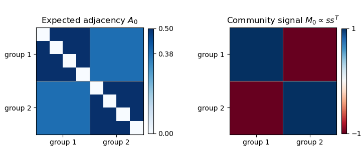
Write $s_i=1$ on $S$ and $s_i=-1$ on $S^c$, and put $v=s/\sqrt{n}$ and $w=1/\sqrt{n}$. Because the two groups have equal size, $v,w$ are orthonormal. Let $a=1/2-t/(2\sqrt{n})$ and $b=t/(2\sqrt{n})$. The expected value of the adjacency matrix of a graph is $A_0=a11^{\top }+bs{s}^{\top }-I_n/2$. ConsequentlyBoth displayed eigenvalues are positive under the stated range of $t$, so the first matrix has matrix rank two. The other $n-2$ eigenvalues are zero. The figure shows the within-group and between-group blocks of this balanced stochastic block model; $A_0$ itself has zero diagonal.

For partitions, the appropriate Hamming distance between unlabelled bipartitions is $\Delta (T,S)=\min \{|T△S|,|T△S^c|\}$. It counts vertices assigned to the wrong group after the better global exchange of the two group names. The printed signed-indicator formula does not implement this exchange: negating a zero-one indicator is not taking its complement. It must be read as this partition distance, or written with the $\pm 1$ membership vectors.

Use the corrected leading eigenvector estimator from 4(b), and orient its sign to minimize $\Vert \hat{v}-\sigma v{\Vert }_2$. At every wrongly signed coordinate, this difference has magnitude at least $1/\sqrt{n}$. Therefore the sign rounding bound for a unit eigenvector givesThe last inequality uses the projector distance bound $\sqrt{2}\le 2$. Taking the expected value of this Frobenius norm estimate proves $\mathbb{E}\Delta (\hat{S},S)\le 2nc/t$. The assertion relies on the corrected estimator and partition-distance definition.

The Kullback-Leibler divergence of a product measure is the sum of the individual divergences, by expanding the logarithm of the likelihood ratio and taking its expected value. Put $q=1/2-t/\sqrt{n}$ and define $W(S)$ to be the unordered pairs lying within one group, while $C(S)$ is the set of unordered pairs crossing between groups. ThenThus choosing the printed $\partial S$ to mean $W(S)$ gives its order of the summands. If $\partial S$ denotes the usual graph cut $C(S)$, their two orders must be interchanged. Each unordered edge is counted once.

The inequality $\log x\le x-1$ givesSince $1/3<q<1/2$, each changed-edge divergence is at most $9t^2/(2n)$. Summing over at most $n(n-1)/2$ pairs gives $D_{\mathrm{KL}}(P_S\Vert P_{S^{\prime }})\le 9n{t}^2/4$. This is the information scale needed for Fano's inequality.

An open migration process is a continuous-time Markov chain recording the populations $n=(n_1,\dots ,n_J)$ of finitely many colonies. Independent external Poisson processes bring individuals to colony $j$ at rate ${\nu }_j$. When that colony contains $k>0$ individuals, a departure opportunity occurs at total rate ${\varphi }_j(k)>0$, with ${\varphi }_j(0)=0$. The departing individual moves to colony $l$ with probability $p_{jl}$, or leaves the system with probability $p_{j0}=1-{\sum }_l{p}_{jl}$. Routing choices and the clocks are independent. A return to the same colony does not change the state.

The word open means that the routing matrix $P=(p_{jl})$ is transient: every individual eventually leaves, or equivalently the spectral radius of $P$ is less than one. The traffic equations of an open migration process, with row-vector convention, give the total arrival rates:These rates include migrations as well as external arrivals. On the active colonies assume ${\alpha }_j>0$ and the usual irreducible Markov chain condition. PutThe product form and its normalization condition areTo establish the product-form stationary distribution of an open migration process, first use its unnormalized weight $b(n)={\prod }_j{b}_j(n_j)$. Its ratios satisfy $b_j(k){\varphi }_j(k)={\alpha }_j{b}_j(k-1)$. The incoming external arrivals into $n$, divided by $b(n)$, contribute ${\sum }_j{\nu }_j{\varphi }_j(n_j)/{\alpha }_j$. Incoming exits contribute ${\sum }_i{\alpha }_i{p}_{i0}$. Incoming migrations from $i$ to $j\ne i$ contribute ${\alpha }_i{p}_{ij}{\varphi }_j(n_j)/{\alpha }_j$. Terms involving an empty destination are zero. Thus the full incoming rate divided by $b(n)$ isHere the traffic equations of an open migration process give the second equality, including ${\sum }_i{\alpha }_i{p}_{i0}={\sum }_j{\nu }_j$. The right side is precisely the total outgoing rate. This proves global balance for a continuous-time Markov chain; pairwise detailed balance is not required for general routing.

For finite rates at each finite population, the continuous-time Markov chain is nonexplosive Markov chain: its total population is bounded over a finite time interval by the initial population plus the finitely many external arrivals, so it visits a finite set on which all jump rates are bounded. Consequently finite $Z_j$ normalize the invariant weight to a stationary distribution. Under the stated irreducible Markov chain assumptions, this is the unique stationary distribution, and it is a positive recurrent Markov chain. Conversely, the unique invariant measure of an irreducible recurrent chain is proportional to $b$, so a positive recurrent Markov chain requires its normalization to be finite. A sufficient condition is ${\mathrm{liminf}}_{k\to \infty }{\varphi }_j(k)>{\alpha }_j$; the series criterion itself is the exact condition. Colonies with ${\alpha }_j=0$ have zero stationary population and can be removed from the active class.

For the single-server M-M-1 queue specialization, ${\varphi }_j(k)={\varphi }_j$ for $k>0$, each stationary colony has the geometric distribution of an M-M-1 queue:The traffic equations of an open migration process do not involve the service rates, so the ${\alpha }_j$ remain fixed during this service-capacity allocation in an open migration process. Write $A={\sum }_j{\alpha }_j$, $B=F-A$ and $b_j={\varphi }_j-{\alpha }_j$. A stationary allocation requires $B>0$, with $b_j>0$ and ${\sum }_j{b}_j=B$. The Cauchy-Schwarz inequality givesEquality holds exactly when $b_j$ is proportional to $\sqrt{{\alpha }_j}$. Hence, for positive arrival rates, the unique optimal service allocation and the minimum expected value of the total population areIf $F\le A$ and some arrival rate is positive, no stable service allocation exists. Zero-arrival colonies need no service in their stationary empty class: allowing zero service there gives the same formula restricted to active colonies. If strictly positive service is demanded even at inactive colonies, the displayed minimum is an infimum approached as that unused allocation tends to zero. If all arrivals vanish, the stationary mean population is zero for every allocation that drains the initial population.

Apply Markov's inequality to the nonnegative random variable $e^{\lambda X}$, since $X>t$ implies $e^{\lambda X}>e^{\lambda t}$:This exponential Markov bound remains true, though uninformative, when the expected value is infinite. For a standard normal distribution, completion of the square gives its moment-generating functionMinimize ${\lambda }^2/2-\lambda t$ over positive $\lambda$; the choice $\lambda =t$ gives the Chernoff bound

Let $C_{12}=\mathbb{E}[S_1{S}_2]\ge 0$, using the supplied correlation property of the Curie–Weiss model. Since $1_{\{S_i=1\}}=(1+S_i)/2$ and each spin has zero expected value,Divide by $\mathbb{P}(S_1=1)=1/2$ to obtainThe expression assumes $n\ge 2$, as required for $S_2$ to exist. It makes the connection between the spin correlation and the requested conditional probability explicit.

Write $K=k+1$ and $h_j={\mathbb{E}}_j{D}_j$. The expected duration of symmetric gambler's ruin satisfies $h_0=h_K=0$ and, by conditioning on the first step,These expected values are finite: from any interior state, $K$ consecutive right steps ensure absorption, an event of probability at least $2^{-K}$. Blocks of $K$ steps therefore bound the survival probability by a decreasing geometric sequence. The candidate $h_j=j(K-j)$ has the required boundary values and satisfies $h_{j+1}-2h_j+h_{j-1}=-2$. HenceFor completeness, the difference of two solutions of this linear recurrence relation has zero second difference and is affine in $j$; its two zero boundary values force it to vanish.

The vertices visited by a simple symmetric random walk form an integer interval: nearest-neighbour steps cannot skip a vertex. At the stopping time $T_k$, write that interval as $[\ell ,r]$, with $r-\ell +1=k$. The walk is at one of its endpoints, because the $k$th new vertex must extend the earlier interval. This also covers $k=1$, when both endpoints coincide.

The Strong Markov property restarts the walk from this endpoint. Visiting a new vertex is exactly exiting $[\ell ,r]$, or reaching $\ell -1$ or $r+1$. Translate these absorbing boundaries to $0,k+1$. The starting point becomes either $1$ or $k$, so the expected duration of symmetric gambler's ruin is $k$ in both cases. Taking conditional expectations and then expected values gives the expected time to expand a random-walk range:

Because $X$ is a nonnegative integer, its indicator function satisfies $1_{\{X>0\}}\le X$. Taking expected values proves the upper bound. The finite second moment also gives a finite expected value, by the Cauchy-Schwarz inequality. Applying that inequality to $X$ and $1_{\{X>0\}}$ givesThe assumed positive second moment permits division, yieldingThe lower bound is the basic second moment method; the upper bound also follows from Markov's inequality at threshold one. Integer-valuedness is essential for that upper bound, but not for the lower bound. For example, a constant $X=1/2$ would violate the upper bound.

The conditional density givesusing either integration by parts or the expected value of an exponential distribution. HenceThis is a finite value for almost every realization of $X$, but not an integrable random variable: $\mathbb{E}[1/X]={\int }_0^{\infty }{e}^{-x}/xdx=\infty$. Since $Y\ge 0$, its conditional expectation remains well-defined in the nonnegative, extended-expectation sense; the tower property of conditional expectation then gives $\mathbb{E}Y=\infty$.

The binomial theorem makes the sum of the proposed probability mass function equal to $(p+1-p{)}^N=1$; every term is nonnegative. Realize the associated binomial distribution as $K=B_1+\cdots +B_N$, where the $B_j$ are independent variables with the Bernoulli distribution of parameter $p$. Each has expected value $p$ and variance $p(1-p)$. Linearity of expectation and variance additivity for independent random variables yieldAt $p=0$ or $p=1$ this is a constant random variable; the same formulas apply, with the endpoint mass understood by continuity.

Use the radial exponential $e^{-\alpha r}$ shown in the original PDF; the TeX's $e^{-\alpha x}$ is a transcription defect. Every orbital angular momentum operator annihilates a radial function, so it acts only on $P=x_1+x_2+2x_3$. The angular momentum of a radial function times a linear polynomial is determined by its degree-one angular factor: direct application of the rotation derivatives givesEquivalently its restriction to the sphere is a degree-one spherical harmonic. ThusFurthermore ${\hat{L}}_3\psi =-i\hslash K(x_1-x_2)e^{-\alpha r}$. Its expected value is proportional to the integral of $(x_1+x_2+2x_3)(x_1-x_2)e^{-2\alpha r}$. The cross terms are odd in a coordinate, and the integrals of $x_1^2$ and $x_2^2$ agree by rotational symmetry. HenceThe state need not be an eigenstate of ${\hat{L}}_3$. If normalization is desired, $\int P^2{e}^{-2\alpha r}{d}^{3}x=6\pi /{\alpha }^5$, so $K={\alpha }^{5/2}/\sqrt{6\pi }$; the zero expectation holds after normalization for any nonzero initial $K$.

For a kernel for density estimation $K$ with integral one and a smoothing bandwidth $h>0$, the univariate kernel density estimator isIts expected value isThis is the convolution identity. It holds wherever the integral is defined, in particular everywhere for the bounded kernel used below. For a nonnegative kernel for density estimation, Tonelli theorem also gives the identity as an extended nonnegative integral. A signed kernel for density estimation instead requires absolute integrability for this interchange.

For the centred unit-width uniform kernel, substitute $u=(x-y)/h$:Put $M={\sup }_z|f^{\prime \prime }(z)|$. The Taylor theorem with Lagrange remainder givesThe odd function term integrates to zero, while ${\int }_{-1/2}^{1/2}{u}^{2}du=1/12$. Hence the bias of a kernel density estimator obeysThis is a second-order pointwise bias bound for kernel density estimation. Existence and boundedness of the second derivative suffice for the stated remainder; continuity of that derivative is not an extra assumption.

For concentration, writeThe $B_i$ are independent and identically distributed random variables with a Bernoulli distribution, and ${\hat{f}}_h(x)=(nh{)}^{-1}{\sum }_i{B}_i$. The required concentration bound follows from the Hoeffding lemma. We prove its Bernoulli case directly. Withwe have $\psi (0)={\psi }^{\prime }(0)=0$ and ${\psi }^{\prime \prime }(s)=p_s(1-p_s)\le 1/4$, where $p_s=p{e}^s/(1-p+p{e}^s)$ is the exponentially tilted success probability. Therefore $\psi (s)\le s^2/8$ for every real $s$. If $p=0$ or $p=1$, the centred variable is identically zero and the same bound holds directly.

Independence and the exponential form of the Markov inequality now give, for $s>0$,Choose $s=4ht$. Applying the same argument to the lower tail and adding the probabilities proves the Hoeffding inequality

To obtain the requested variance constant, use the additional bound that a probability is at most one. Set $Z={\hat{f}}_h(x)-\mathbb{E}{\hat{f}}_h(x)$ and $a=2n{h}^2$. The tail integral formula for moments, justified by Tonelli theorem, yieldsThusThe clipping at one is essential for this integration argument to give that constant. It is an instance of a second moment bound from a clipped Gaussian tail. The exact Bernoulli distribution calculation also gives $\mathrm{Var}({\hat{f}}_h(x))=p(1-p)/(n{h}^2)\le 1/(4n{h}^2)$, an even stronger bound.

Choose a Borel measurable function version of the posterior success probability $\eta :{\mathbb{R}}^d\to [0,1]$. Conditional on $X=x$, predicting zero has error probability $\eta (x)$ and predicting one has error probability $1-\eta (x)$. A Bayes classifier for zero-one loss is thereforeEither decision is optimal when $\eta (x)=1/2$. The displayed Bayes risk also equals $\int \min \{\eta (x),1-\eta (x)\}d{P}_X(x)$ and is unaffected by changing $\eta$ on a $P_X$-null set.

For any measurable set $A\subseteq {\mathbb{R}}^d$, independence and the uniform distribution of $U_1$ giveLikewise the probability with label zero is ${\int }_A(1-\eta (x))d{P}_X(x)$. These sets determine the joint probability distribution, soThe same construction makes all training pairs independent and identically distributed random variables.

Fix a feature-measurable nearest-neighbour tie-breaking rule, for example increasing original index for observations at equal Euclidean norm distance from the query. This is important: the ordering may depend on the features, but not on the $U_i$ or labels. Let $Y_{(j)}(x)$ be the label attached to the $j$th ordered feature. The classifier from the K-nearest neighbors algorithm isThe displayed rule resolves a tied vote in favour of one; any fixed vote convention would also define the method. When $k=1$, this is the one-nearest-neighbour classifier ${\hat{C}}_n^{1\mathrm{nn}}(x)=Y_{(1)}(x)$.

Write $I_n(x)$ for the selected original index. Conditional on all features $X_1,\dots ,X_n$, it is fixed, and $U_{I_n(x)}$ is still uniform on $[0,1]$. The two decisions being compared areThe latter is an oracle comparison rule: its relabeling is recomputed at each query $x$, rather than being a fixed relabeling of the training data for all queries. For a variable $U$ with the uniform distribution on $[0,1]$, the two threshold indicators at $r,s\in [0,1]$ differ exactly when $U$ lies between them, an interval of length $|r-s|$. This Bernoulli coupling by a shared uniform random variable proves

Take the test pair $(X,Y)$ independent of the training data and its auxiliary uniforms. Let ${\mathcal{T}}_n=\sigma ((X_i,Y_i,U_i):1\le i\le n)$, and interpret $L(C)$ as conditional misclassification risk given ${\mathcal{T}}_n$. The tower property of conditional expectation gives $\mathbb{E}L(C)=\mathbb{P}(C(X)\ne Y)$. Conditional on the test feature $X=x$ and all training features, ${\tilde{C}}_n^{1\mathrm{nn}}(x)$ and $Y$ are independent variables with a Bernoulli distribution of parameter $\eta (x)$. Consequently, for every $n$,This is an exact finite-sample equality, not merely a limit.

The two error indicators can differ only if the two classifiers disagree, soThe permitted nearest-neighbour approximation theorem states that the last expected value tends to zero for the feature-based selection rule. This establishes the one-nearest-neighbour asymptotic risk

For $r\in [0,1]$, put $a=\min (r,1-r)\in [0,1/2]$. Then $2r(1-r)=2a(1-a)$, and $a\le 2a(1-a)\le 2a$. Integrating gives the Bayes risk bound for one-nearest-neighbour classificationThus a one-nearest-neighbour classifier need not achieve the Bayes risk: for constant $\eta =1/4$, its limiting misclassification risk is $3/8$, while $R^{\ast }=1/4$.

Feature-based neighbour tie-breaking is required. The convention cannot be dropped for arbitrary $P_X$. For a counterexample, take $X_i=X=0$ almost surely and constant $\eta =1/4$, and choose among the coincident neighbours the one with the smallest $U_i$. Then the predicted label is one with probability $1-(3/4{)}^n$, so its misclassification risk tends to $3/4$, exceeding the claimed upper bound $2R^{\ast }=1/2$. The corrected theorem uses ties determined independently of the uniforms and labels, as above.

Use simple random walk on the loopless undirected unweighted graph, with transition probability $1/\mathrm{deg}(x)$ to each graph neighbour, and take $a\ne z$. Set $T_z=\inf \{t\ge 0:X_t=z\}$. Returns to $a$ before visiting $z$ do not end the commute. After its first visit to $z$, stop at the subsequent first visit to $a$, so $\tau =T_z+T_a\circ {\vartheta }_{T_z}$. Count transitions with departure times $0\le t<\tau$, including the final step arriving at $a$. The expected hitting times are finite: in a finite connected graph there is a uniformly positive probability to reach any fixed target within a fixed number of steps, giving a geometric tail bound.

We prove the needed killed-walk occupation voltage identity from its visit balance equation. DefineFor $x\ne z$, counting arrivals before absorption givesHence, for the Graph Laplacian $Lv(x)=\mathrm{deg}(x)v(x)-{\sum }_{y\sim x}v(y)$, we have $Lv(x)=1_{\{x=a\}}$ away from $z$. Since the sum of all Laplacian coordinates is zero, $Lv(z)=-1$. Thus $v$ is the electrical voltage of a unit flow from $a$ to $z$, grounded at $z$, and $v(a)=R_{\mathrm{eff}}(a,z)$.

Construct $w(x)=g_{za}(x)/\mathrm{deg}(x)$ for the opposite killed leg. It satisfies $Lw={\delta }_z-{\delta }_a$ and $w(a)=0$. Therefore $L(v+w)=0$. The harmonic maximum principle on a finite graph makes $v+w$ constant: at a maximum its value equals the average over its graph neighbours, forcing all of them to share that value, and connectedness propagates it. At $a$ the constant equals $R_{\mathrm{eff}}(a,z)$.

For any oriented edge $(x,y)$, each visit to $x$ before the target hit produces a transition to $y$ with conditional probability $1/\mathrm{deg}(x)$. The expected traversals during the first killed leg are therefore $v(x)$, and those during the second leg are $w(x)$ by the Strong Markov property at $T_z$. This proves directed edge occupation in a random-walk commute:In particular, both directions of every unoriented edge have this same expected value, although their counts on an individual commute need not coincide. Summing over the $2|E|$ directed edges also recovers the commute time identity ${\mathbb{E}}_a\tau =2|E|R_{\mathrm{eff}}(a,z)$.

The distinct-terminal convention is necessary for the printed “returns” interpretation. If $a=z$ and $\tau$ is the first positive return, a graph with two graph vertices and one edge gives $S(a,y)=1$ while $R_{\mathrm{eff}}(a,a)=0$. Thus either take $a\ne z$, as intended, or explicitly define the degenerate commute as $\tau =0$. A general nonuniform random walk is not covered by the unweighted simple-walk formula.

Group the random resistance cost by unoriented edges. For $e=\{x,y\}$, its resistance contributes once whenever the walk traverses it in either direction. Pathwise,The graph is finite and the commute has finite expected value. Linearity of expectation, or Tonelli theorem for these nonnegative terms, therefore permits taking expectations of the sum. By the directed edge occupation in a random-walk commute, both directed traversal counts have expected value $R_{\mathrm{eff}}(a,z)$. ThusApply Foster's theorem from part (a) to obtainThe factor two counts the two orientations of each edge. It would be lost by treating the expected directed count in part (b) as an expected count for both directions together. The same distinct-terminal and simple-random-walk conventions from part (b) remain in force.