Flows, fluctuations and complexity and symmetry and relativity paper of Part B of the physics course of the University of Oxford (B1)

Source paper: www-thphys.physics.ox.ac.uk/people/AndreiStarinets/TUTORIAL_NOTES_SR/exam_2011_symmetry_relativity.pdf

Section I comprises questions 1–4; Section II comprises questions 5–8. Numbered subdivisions below retain the successive unlettered source blocks; letters retain the source's actual letters. The Symmetry and Relativity 2011 Exam Solution Notes answer much of Section II. Covered requests are linked to their precise pages; supplements below fill requests omitted or only referred elsewhere. These page references describe coverage, not an independent certification of every calculation in the notes.

Set ${\partial }_t\mathbf{u}=0$ and $\nu =0$ in the Navier-Stokes equation. Dotting the resulting Euler equation with a displacement $d\mathbf{r}$ tangent to a streamline givesHere mass density $\rho$ is constant, and $B$ is constant along each streamline. The terms are kinetic energy per unit mass, the pressure work per unit mass available from pushing a parcel through the flow, and gravitational potential energy per unit mass. Their sum is conserved mechanical energy per unit mass; $p/\rho$ is not an additional independently conserved parcel energy. Different streamlines can have different $B$ unless, for example, the flow is also irrotational in a connected region.

For planar incompressible flow, $u_x+w_z=0$. Locally this permits a streamfunction with $u={\psi }_z$, $w=-{\psi }_x$, because equality of the mixed derivatives enforces incompressibility. The remaining component of the curl is $u_z-w_x={\psi }_{zz}+{\psi }_{xx}$, so irrotational flow requires Laplace's equation for $\psi$.

Put $K=\pi /b$. The sinusoidal contribution to the supplied streamfunction has ${\psi }_{xx}=U_{0}a{K}^2\cos (Kx)e^{-Kz}$ and ${\psi }_{zz}=-U_{0}a{K}^2\cos (Kx)e^{-Kz}$; the linear term is also harmonic. HenceAs $z\to \infty$, these approach the specified uniform flow, $(u,w)=(U_0,0)$.

The impermeability kinematic boundary condition is $w=u{z}_s^{\prime }(x)$ on $z=z_s(x)$, equivalently $\psi$ is constant on the wall. For $aK\ll 1$, evaluating the perturbed velocities at $z=0$ gives $w=-U_{0}aK\sin (Kx)=U_0{z}_s^{\prime }$ to first order. The residual is of order $U_0(aK{)}^2$. Equivalently $\psi (x,z_s)=U_{0}a\cos (Kx)[1-e^{-Ka\cos (Kx)}]=O(U_{0}K{a}^2)$. The surface velocity isThe first expression is the supplied approximate field evaluated exactly at the wall; its accuracy as a wall-flow solution is still only first order in $a/b$.

Use the rest frame of the hydrofoil, with undisturbed velocity $U_0{\mathbf{e}}_x$. Let $p_{\ast }$ be the undisturbed pressure at the lower surface level $z=0$, so the undisturbed hydrostatic pressure is $p_{\ast }-\rho gz$. The Bernoulli equation gives, with $h=a\cos (\pi x/b)$ and $ϵ=\pi a/b$,These formulas implement the prescribed neglect of the other velocity components. To the controlled first order in $a/b$, $p_{\mathrm{lower}}-p_{\mathrm{upper}}=\rho gh+\rho U_0^2ϵ\cos (\pi x/b)$. The vertical component of pressure acting on an inclined surface is integrated over its horizontal projection, soThe total upward fluid force per unit span is $L_{\mathrm{dynamic}}^{\prime }+B^{\prime }$. The lift due to motion is $L_{\mathrm{dynamic}}^{\prime }$; $B^{\prime }$ is the separate buoyancy. If the given approximate speed is squared without truncation, the formal additional dynamic term is $\rho U_0^2{\pi }^2{a}^2/(4b)$, but a controlled second-order prediction would require the omitted second-order flow and transverse-velocity contributions too.

Take positive circulation to mean counterclockwise in the $(x,z)$ diagram, with $x$ right and $z$ up. The upper surface is then traversed right to left. To first order in $a/b$,Thus the bound circulation is clockwise. Any exterior contour enclosing the hydrofoil has the same circulation in an irrotational flow; a globally completed two-dimensional flow must contain a circulation component decaying as $|\Gamma |/(2\pi r)$ at large distance. The simple local upper/lower velocity prescription cannot describe the entire exterior. For a start from rest, Kelvin's circulation theorem requires compensating shed vorticity, represented by a starting vortex in a physical wake.

Numerically,If the question's fluid force includes buoyancy, $B^{\prime }\simeq 1.25\times 10^3\mathrm{N}{\mathrm{m}}^{-1}$ and the total upward fluid force is about $2.05\times 10^3\mathrm{N}{\mathrm{m}}^{-1}$, using $g=9.81\mathrm{m}{\mathrm{s}}^{-2}$. Weight of the hydrofoil is not specified and is not part of this fluid force. The motion-induced lift also agrees with the Kutta–Joukowski theorem, $L^{\prime }=-\rho U_0\Gamma$ in this orientation.

The chord-based Reynolds number isAt this large Reynolds number, smooth laminar flow over the whole body is unlikely in ordinary conditions; wall layers may undergo transition and separate. A thin-layer inviscid flow approximation outside them can remain useful, but does not justify globally laminar flow.

Write $\mu$ for dynamic viscosity and $\nu =\mu /\rho$ for kinematic viscosity, consistently with the introductory Navier-Stokes equation. The phrase “dynamic viscosity $\nu$” in this request mixes these conventions. A fully developed plane Poiseuille flow, $\mathbf{u}=(u(z),0,0)$, has zero convective acceleration. The Navier-Stokes equation gives $\mu u^{\prime \prime }=-f$ and $p_z=-\rho g$. Applying the no-slip boundary condition at both stationary plates givesThe material coefficients must be effectively constant and positive. The profile is an exact parallel-flow solution for every $\mu >0$; experimental validity additionally requires that the realized flow remain in the laminar flow regime. A sufficient conservative condition isEquivalently $\nu \gg \sqrt{f{b}^3/(12\rho )}$, or $\mu \gg \sqrt{\rho f{b}^3/12}$. This sufficient bound is stronger than necessary; there is no need to discard convective acceleration by an approximation here because it vanishes identically for the assumed profile.

Here $k$ is a mass absorption coefficient, because $k\rho$ has units of inverse length. The Beer-Lambert law is $dF/dz=-k\rho F$, giving $F(z)=F_0{e}^{-k\rho z}$. A horizontal slab of area $A$ and thickness $dz$ absorbs power $A[F(z)-F(z+dz)]$. Dividing by its volume and taking the limit gives

A parcel at fixed $z$ spends time $a/u(z)$ in the light. With no thermal conduction or thermal expansion, its energy balance is $\rho cdT/dt=q_R$. Equivalently the steady advection equation is $\rho cu(z)T_x=q_R(z)$ with $T(0,z)=T_0$. ThereforeThe no-slip boundary condition makes residence time diverge as either wall is approached. The resulting unbounded temperature is a failure of the approximations, rather than a physically steady wall prediction. Even small thermal conductivity transfers heat away from these layers; conduction into real perspex adds another heat sink. Thermal expansion can alter mass density, create buoyancy-driven motion and change the background profile, while temperature-dependent dynamic viscosity changes the assumed residence time. With exactly insulating walls, finite fluid thermal conductivity still regularizes the transverse profile; an entrance region and, sufficiently near a stagnant wall, longitudinal conduction also matter.

Put $A=2\mu a{F}_{0}k/(cf)$. In the specified near-wall limit the outer temperature is $T-T_0\simeq A/(bz)$, soThus the near-wall radiative heating layer has scaleThe comparison is an estimate of the breakdown of the outer solution, not a new inner temperature solution. It requires ${\delta }_C\ll b$ and $k\rho {\delta }_C\ll 1$; neglecting longitudinal relative to transverse thermal conduction additionally requires ${\delta }_C\ll a$ in the region to which the estimate is applied.

An equilibrium point of a dynamical system is a state ${\mathbf{x}}_{\ast }$ with $\mathbf{f}({\mathbf{x}}_{\ast })=0$, so the trajectory stays there. In a planar phase portrait, an unstable spiral has a complex-conjugate pair of Jacobian matrix eigenvalues with positive real part: nearby trajectories rotate while moving outward. An attractor is an invariant set approached by trajectories from a neighborhood, its basin of attraction. It can be an equilibrium point, a limit cycle, or a more complicated set; outward spiralling near one equilibrium point does not preclude attraction to a larger set.

At an equilibrium point of the Rössler system, $y=-z$, $x=az$, and $a{z}^2-cz+a=0$. HenceThere are two distinct real equilibrium points only if $c>2a$; they merge if $c=2a$ and there are none if $c<2a$. Positivity of $a,c$ alone does not guarantee two. Under the later limits, the nearer one is $(x_{-},y_{-},z_{-})\simeq (a^2/c,-a/c,a/c)$, while $(x_{+},y_{+},z_{+})\simeq (c,-c/a,c/a)$.

The Jacobian matrix of the Rössler system isAt the origin the vertical homogeneous perturbation obeys $\delta \dot{z}=-c\delta z$, so it decays as $e^{-ct}$. Nearby, $\dot{z}\simeq a-cz$ also relaxes the trajectory toward $z\simeq a/c$, close to the $x$–$y$ plane. The small fixed-point value of $z$ weakly couples planar errors back into $z$; this is neglected in the requested approximation.

The planar block has trace $a$ and determinant $1$, withFor $0<a\ll 1$, this is an unstable spiral. Writing $X=x-x_{-}$ and $Y=y-y_{-}$, its linearized trajectories have an envelope proportional to $e^{at/2}$ and angular frequency approximately $1$. They rotate counterclockwise: at $X>0,Y=0$, $\dot{Y}=X>0$. Fast vertical contraction occurs on scale $1/c$, much shorter than the planar growth scale $2/a$.

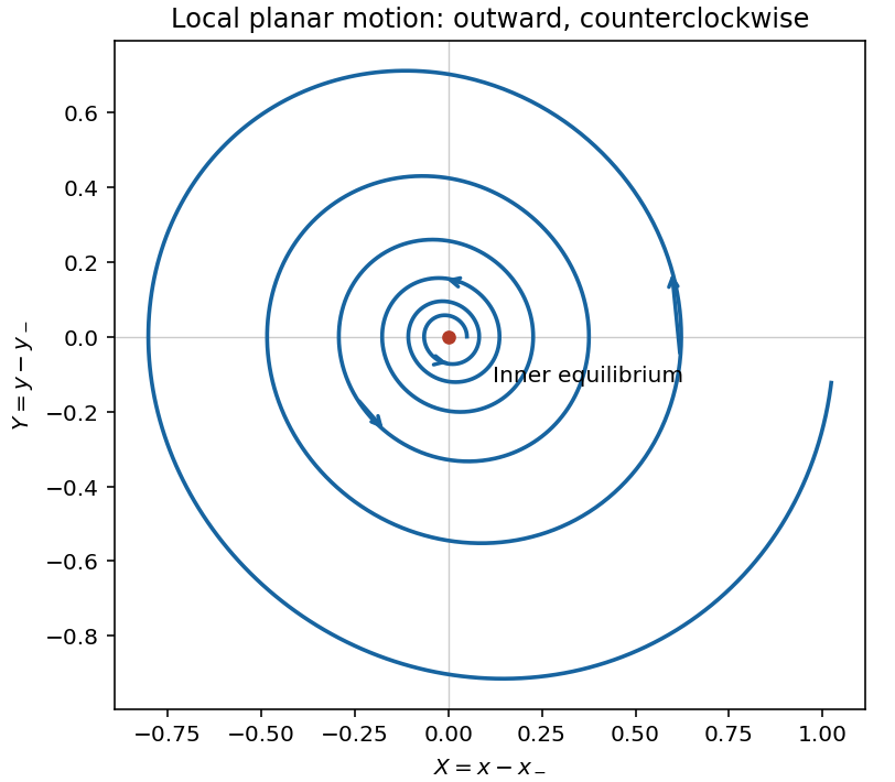
Confinement weakens as $x$ approaches $c$ from below; the approximate vertical relaxation time is $1/(c-x)$, and the quasi-steady value $a/(c-x)$ ceases to be small. For $x>c$, the coefficient of $z$ becomes positive, so vertical departures are amplified. The plane $z=0$ is never exactly invariant because $\dot{z}=a$ there.

For an infinitesimal perturbation $\mathbf{\eta }$, $\dot{\mathbf{\eta }}=J\mathbf{\eta }$, andThus the principal instantaneous stretching rates, called local Lyapunov exponents in the question, areFor $z\ne 1$, ${\lambda }_{+}>0$ and ${\lambda }_{-}<0$, while $a>0$. There are two instantaneously expanding orthogonal directions and one contracting direction. These are instantaneous norm-growth rates; the directions rotate along a trajectory, so this does not imply two positive long-time Lyapunov exponents or indefinitely exponential growth along fixed axes.

At $x=c$, put $s=\mathrm{sgn}(z-1)$. The eigenvectors and rates areThe condition $|z-1|>2a$ makes ${\mathbf{e}}_{+}$ the fastest-growing direction, faster than ${\mathbf{e}}_y$; ${\mathbf{e}}_{-}$ is the fastest-contracting direction. Both lie at $45^{\circ }$ to the $x,z$ axes.

Take $u>0$. Despite the source's terminology, $P(x)$ is a dimensionless conditional bound-state probability at phase $x$, not a spatially normalized probability density; the phase-average bound fraction is ${\Delta }^{-1}{\int }_0^{\Delta }Pdx$. The given equation has advection and binding reactions but no diffusion term. Large $N$ permits the prescribed steady $u$ approximation.

For spatially gated myosin attachment, define $A=e^{-k_1{x}_1/u}$, $B=e^{-k_2(\Delta -x_2)/u}$, $p_0=P(0)$ and $p_b=P(x_1)$. Continuity and periodicity give $p_b=1-(1-p_0)A$, $p_0=B{p}_b$, hence $p_b=(1-A)/(1-AB)$. The full periodic steady solution isThe requested limit makes $B\ll 1$, so $p_0\simeq 0$ and $p_b\simeq 1-e^{-k_1{x}_1/u}$. The curve rises exponentially over the binding window, remains flat to $x_2$, then decays over length $u/k_2$ to an exponentially small value before the next period. The piecewise expression is continuous at both switching points and at the period boundary.

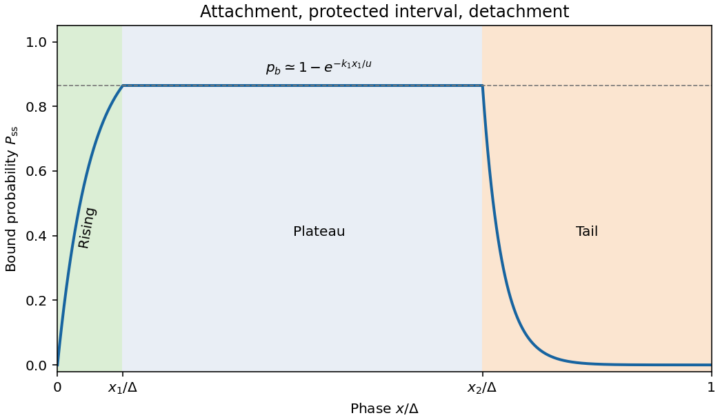
For a head sampling phases uniformly during steady sliding, its mean force is $f_0$ times the phase-average bound probability. In the $B\ll 1$ limit of spatially gated myosin attachment, integrating the three intervals givesThe first integral is bounded by $x_1{p}_b$, and the last by $(u/k_2)p_b$. Relative to the plateau contribution, they are negligible when $x_1\ll x_2$ and $u/k_2\ll x_2$, respectively. ThereforeThis is a constant-force spatially gated motor approximation: complete detachment between binding windows, a narrow attachment window, a short detachment tail and essentially fixed sliding velocity. In particular, $k_1{x}_1/u$ need not be small.

Put $V=k_1{x}_1$ and $F_{\ast }=N{f}_0{x}_2/\Delta$. The constant-force spatially gated motor producesThe limit is approached after the periodic steady state is established; at exactly $u=0$ arbitrary initially bound heads in inactive phase intervals need not equilibrate. The curve decreases from $F_{\max }$ and has formal large-$u$ tail $F_{\max }V/u$. Extrapolation of that tail beyond the small-$u$ detachment assumptions is not controlled.

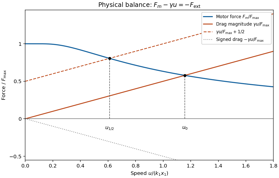
Sign inconsistency in the printed force balance. For a positive viscous drag coefficient $\gamma$, the signed drag force is $-\gamma u$. The printed $F_{\mathrm{ext}}+F_m+\gamma u=0$ cannot give the requested positive no-load contraction speed: both last terms are positive when $u>0$. With $F_{\mathrm{ext}}=-F_{\max }/2$, the left side starts at $F_{\max }/2>0$ and may have zero, one or two positive roots depending on parameters; the requested usual load construction is not implied by that equation.

The physical linear-drag load curve for a spatially gated motor usesOn the same axes plot the positive drag magnitude $D(u)=\gamma u$ and the decreasing motor force $F_m(u)$. The no-load speed $u_0$ is their intersection. For opposing load $F_{\max }/2$, intersect $F_m(u)$ with the parallel raised line $D(u)+F_{\max }/2$; equivalently intersect $D(u)$ with $F_m(u)-F_{\max }/2$. Drop verticals to the speed axis. The loaded speed obeys $0<u_{1/2}<u_0$. Each intersection is unique because $F_m$ decreases and $D$ increases. The signed drag is also indicated below the axis in the sketch.

Covered by the official notes: proper time, rapidity, proper acceleration, longitudinal acceleration transformation, rapidity derivative and additivity (PDF pp. 6–7; handwritten pp. 1–2).^[ref]

Covered by the official notes: onboard acceleration from rearward photon emission (PDF pp. 7; handwritten pp. 2).^[ref]

Covered by the official notes: launch-pad speed as a function of launch-pad time (PDF pp. 8; handwritten pp. 3).^[ref]

Covered by the official notes: mirror-driven acceleration and comparison of the two spacecraft (PDF pp. 8–9; handwritten pp. 3–4).^[ref]

Covered by the official notes: centre-of-momentum energy and momentum of particle 2 and boost speed (PDF pp. 10–11; handwritten pp. 5–6).^[ref]

Covered by the official notes: forward collinear laboratory energy (PDF p. 11; handwritten p. 6).^[ref]

Covered by the official notes: transverse-emission laboratory energy and laboratory angle (PDF p. 11; handwritten p. 6).^[ref]

Covered by the official notes: forward neutrino energy for the specified kaon beam (PDF p. 12; handwritten p. 7).^[ref]

Covered by the official notes: transverse-emission neutrino energy and laboratory angle (PDF p. 12; handwritten p. 7).^[ref]

Covered by the official notes: comparison with a 200 keV neutrino mass (PDF p. 12; handwritten p. 7).^[ref]

The notes stop at “no change”; the experimental implication is that this is a poorly conditioned neutrino mass measurement. In relativistic two-body decay, the corrections to the rest-frame energy and momentum enter through the square of the daughter rest mass, while the Lorentz transformation boosts both the massless value and its small correction. A measured laboratory energy or angle must therefore resolve a very small change against beam-energy spread, decay-angle uncertainty and detector resolution. No visible change at the quoted precision does not establish zero neutrino mass.

The official notes give only “Part 1: as in textbooks” (PDF p. 13, handwritten p. 8). The requested derivation is supplied here.

Put a light source at the rod midpoint in its rest frame $S$ and emit two pulses simultaneously toward its ends, each a distance $\ell$ away. In $S$, the reflection events are $(t,x)=(\ell /c,\pm \ell )$. Invariance of light speed, the Einstein's principle of relativity and linearity give a Lorentz transformation $x^{\prime }=A(x-vt)$, $t^{\prime }=A(t-vx/c^2)$. Applying the inverse transformation with speed $-v$ gives $A^2(1-v^2/c^2)=1$, hence $A=\gamma$.

The transformed reflection events haveThese events are not simultaneous in $S^{\prime }$. Both rod ends move at $-v$ there, so extrapolating each endpoint to $t^{\prime }=0$ gives $x_{\pm }^{\prime }(0)=x_{\pm }^{\prime }+v{t}_{\pm }^{\prime }=\pm \ell /\gamma$. Measuring simultaneous endpoints therefore yields length contraction:

Covered by the official notes: definition of a pure force via constant rest mass (PDF p. 13; handwritten p. 8).^[ref]

The page labels $d{p}^{\mu }/d\tau$ as a proper force; that is the four-force. The requested proper force is the three-force measured in the instantaneous rest frame of the object. For a pure force its magnitude is $m_0$ times the proper acceleration, and in that frame the four-force has components $(0,{\mathbf{f}}_0)$.

Covered by the official notes: longitudinal three-force transformation (PDF p. 13; handwritten p. 8).^[ref]

Covered by the official notes: transverse three-force transformation (PDF p. 13; handwritten p. 8).^[ref]

Covered by the official notes: spring constant parallel to the boost (PDF p. 13; handwritten p. 8).^[ref]

Covered by the official notes: spring constant orthogonal to the boost (PDF p. 13; handwritten p. 8).^[ref]

The orientation-dependent results in the official notes show that the measured spring constant is not a Lorentz scalar. A Lorentz transformation changes both the simultaneous extension and the measured three-force; their ratio depends on the orientation. This does not make the spring intrinsically anisotropic in its own rest frame, or require a preferred inertial frame. It is a quasistatic effective stiffness comparison between frames; an extended real spring also has finite internal signal speeds.

Covered by the official notes: charge field-line sketches at rest and in motion, field anisotropy, and relation to the two spring orientations (PDF pp. 13–14; handwritten pp. 8–9).^[ref]

Covered by the official notes: definitions of four-force and four-velocity and the vanishing antisymmetric contraction (PDF p. 15; handwritten p. 10).^[ref]

To make the necessity statement precise, mass preservation must hold for every allowed timelike four-velocity, with the same field tensor and nonzero charge. It is not necessary for one prescribed trajectory alone. Use metric signature $(-,+,+,+)$, so $U_a{F}^a=-c^{2}dm/d\tau$. Put $H^{ab}=({\mathcal{F}}^{ab}+{\mathcal{F}}^{ba})/2$. The mass-preservation condition requires the quadratic form $H^{ab}{U}_a{U}_b=0$ for every timelike $U$. Every timelike vector can be rescaled to a physical four-velocity; by homogeneity the quadratic form vanishes on the open timelike cone. A polynomial vanishing on an open set is identically zero, so $H^{ab}=0$. Thus the electromagnetic field tensor must be antisymmetric under this universal quantifier. For a single velocity, the scalar contraction can vanish even for a nonzero symmetric part, which is why the quantifier is essential.

The official notes state only ${\mathcal{F}}^{\prime }=\Lambda \mathcal{F}{\Lambda }^T$ (PDF p. 15, handwritten p. 10); they do not evaluate the requested coefficients. For a boost along positive $x$, use ${\Lambda }^0{}_0={\Lambda }^1{}_1=\gamma$, ${\Lambda }^0{}_1={\Lambda }^1{}_0=-\gamma v/c$, with the transverse diagonal entries equal to one. Multiplying the specified electromagnetic field tensor givesThe corresponding Lorentz transformation of electromagnetic fields isConsequentlyThese coefficients depend on the frame speed, but are constant for the fixed boost.

Covered by the official notes: explicit field contraction and Lorentz invariance as a tensor scalar (PDF pp. 15–16; handwritten pp. 10–11).^[ref]

Covered by the official notes: rocket-frame electric and magnetic fields, proper three-force and proper acceleration (PDF p. 16; handwritten p. 11).^[ref]