Consider successive independent Bernoulli trials with the same success probability . A geometric distribution models waiting for their first success. Two conventions coexist, so always say what is counted. Let count all trials up to and including the successful trial, and let count preceding failures. Their probability mass functions areThe factors describe failures followed by one success; independence permits multiplication. Summing the geometric series verifies that each law has total mass one. Their expected values differ by one, while shifting by a constant leaves the variance unchanged:The positive convention and these moments are also given by Penn State STAT 414.[ref]
11 Geometric and Negative Binomial Distributions. STAT 414: Introduction to Probability Theory at Pennsylvania State University; §11.1, Definition 11.1; §11.2, mean and variance theorems
For a constructed retry mechanism with independent attempts and , success on attempt four has probability . More than four attempts are needed precisely when the first four fail: . The expected values are and , and the common variance is . The large spread explains why the average waiting count is not a deadline.
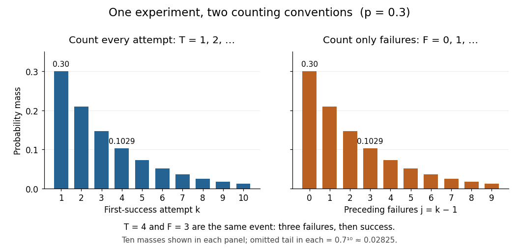
First-success trial versus preceding failures: the same probability masses shifted by one
. Details. 
The two probability mass functions have identical heights with different labels: and describe the same event. For , consecutive masses have ratio , explaining the name geometric distribution. The support of a probability distribution is the positive integers for and the nonnegative integers for . At , it collapses to and , both with variance zero; interpret an empty product, including , as one. These counts concern attempts; converting them into elapsed time requires specifying the time spent per attempt.
The survival function makes the counting convention especially visible. Put . For nonnegative integers , and for ,The event requires failures, whereas requires only when . For the constructed mechanism, differs from . The geometric success deadline uses the latter tail to control the chance of still waiting.
The striking memorylessness of the geometric distribution says that, for nonnegative integers with ,After five failures, the conditional probability of requiring more than two additional attempts is still . The analogous zero-based identity uses ; keeping the inequalities straight avoids an off-by-one error. This property follows from fresh independent trials with unchanged ; learning or changing conditions can destroy it. At , success never occurs, so there is no proper finite waiting-count law.
For independent positive-support geometric random variables with success probabilities , all must exceed for their minimum to exceed . The resulting survival function is . This is the positive-support geometric distribution with the displayed success probability. Independence is needed for multiplying the survival probabilities.
The same argument works for any integer base . Suppose has geometric distribution , , with . Its Euclidean division gives and . Their joint probability mass function isThe factors are normalized probability mass functions, so the final digit and quotient are independent. The quotient again has geometric distribution, with success probability . If is the integer part of an exponential random variable of rate , take .
Suppose a contest uses trials initially and ends there with probability . Conditional on an initial tie, independent further rounds each use trials and resolve the contest with a fixed probability . The number of further rounds, conditional on that tie, has a geometric distribution: for . Thus the total number of trials has an atom at and the displayed probabilities thereafter. The geometric series sums to , so termination has probability one, and the expected value is . The displayed distribution requires independence of the future rounds from the initial tie.
For the positive-integer geometric distribution with success probability , the displayed identity holds for nonnegative integers whenever the conditioning event has positive probability. The first attempts have failed; future independent attempts use the same success probability. Equivalently, divide the tail by . For a zero-based failures count , use . Constant success probability and independence are essential: accumulated wear or learning would require a different model.
The full remaining-count law is unchanged, not only one tail probability. With , after failures set on the event . For , its probability mass function under this conditional probability isHere independence makes the future trials unaffected by the observed failures, and the unchanged success probability makes their law identical to the original one. Consequently , while . For the constructed mechanism, five failures leave a mean of more attempts, making the conditional mean total ; the five already spent are still counted.
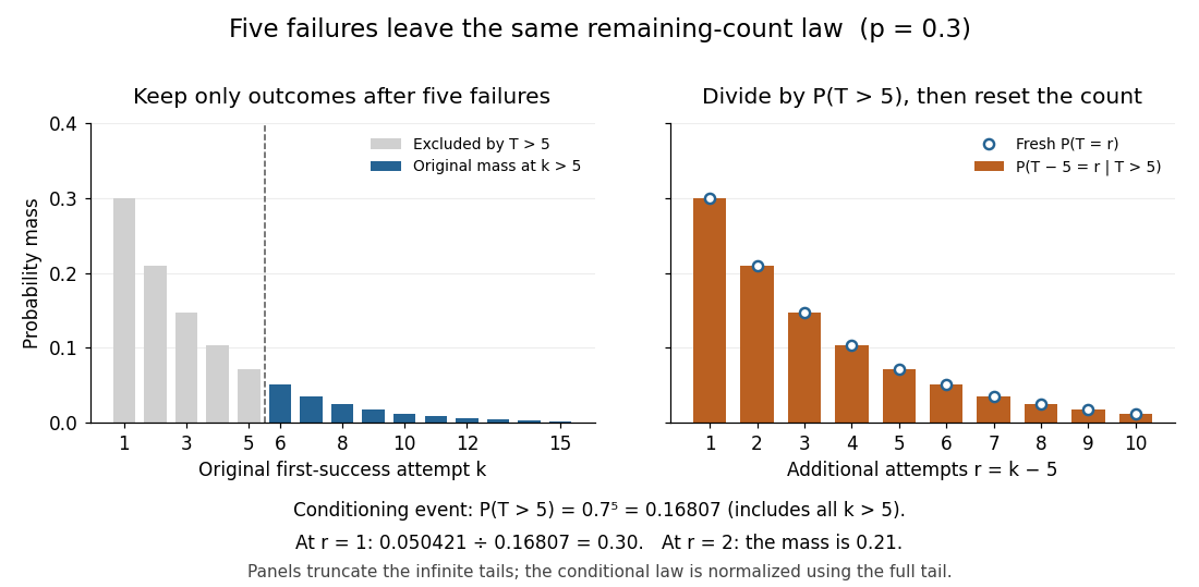
Conditioning on five failures, renormalizing, and resetting the count gives the original geometric law
. Details. 
The same mechanism has constant discrete hazard:Thus each reached attempt has the same chance of success. This differs from the decreasing unconditional probability : later success requires surviving earlier attempts. At , only conditioning on an event of positive probability is allowed: permits only , and only .
Among proper laws on the positive integers, memorylessness of the geometric distribution also characterizes the geometric distribution. Write . The identity gives ; if , both sides vanish anyway. Since , induction yields . Properness excludes , so setting recovers the geometric distribution, including .[ref]
The Geometric Distribution. Random: Probability, Mathematical Statistics, Stochastic Processes by Kyle Siegrist; Basic Theory, Distribution Functions and the Memoryless Property: conditional remaining-count identity and its converse
The retry example stipulates independent Bernoulli trials with a known constant ; it is not evidence that a real retry system behaves this way. Shared changing conditions or adapting attempts can alter the next success probability. Even constant individual success probabilities alone do not imply independence.
For an original contrasting model, uniformly shuffle one success card and three failure cards, then draw by sampling without replacement. Its success position has the discrete uniform distribution on . Initially the success probability is ; after one failure it is . In particular,This shows concretely why sampling without replacement need not be independent and why the remaining wait can change. Every draw still has unconditional success probability when all four positions are considered; the relevant discrete hazard changes after failures.
How many attempts give at least a chosen success probability ? For a positive-integer geometric distribution with , completion by attempt means , soThe logarithm is negative, which reverses the inequality when dividing. The least integer meeting the target is therefore obtained with the ceiling function:For our constructed independent retry mechanism with and ,To verify minimality directly, eight attempts give , whereas nine give . Under the zero-based convention, the same completion event is , with failure to complete given by ; saying would allow ten attempts. A 95% deadline controls a tail probability, while the expected value describes an average.
At success occurs on the first attempt, so ; the logarithm formula is inapplicable. At no finite deadline achieves a positive target. For , no finite deadline guarantees success with probability one because . A retry cap at produces the capped geometric waiting time as the number of attempts actually spent; reaching the cap can mean either success on the last allowed attempt or failure of all attempts.
Start a Markov chain at a nonabsorbing state . If each departure from has probability of absorption before the next return, the Strong Markov property makes the number of visits to , including the initial one, a positive-integer geometric random variable of parameter . For a continuous-time Markov chain whose holding times at are independent rate- exponentials, independently of the embedded jump chain, the total occupation time at is a sum of such holding times and has expected value .
Independently retain each event of a zero-based geometric distribution count with probability . Conditional on the original count, the retained count is binomial, so its probability generating function is . This is again a zero-based geometric distribution, with success parameter and mean . In excess of loss reinsurance, is the probability that a claim exceeds the retention.
Let for and , with . Write . Summing the joint probability mass function with the differentiated geometric series identity gives . By Bayes' theorem,Thus , given , has the failure-count negative binomial distribution for successes and success parameter . Its conditional expectation is for itself. The shift by , the number of retained successes, must be retained when identifying the posterior distribution.
For a positive-integer geometric distribution with , the capped time has masses for and at . The last mass includes all later arrivals, not only . Its probability generating function and expected value areThe expectation follows either by differentiating the PGF or summing the tail probabilities up to .
When independent uniform draws are made from types, the time until every type has appeared decomposes as a sum of independent geometric waiting times with parametersConsequentlyand Chebyshev's inequality gives in probability.
For independent coupon labels arriving at rate , Poisson thinning makes the type-specific first arrival times independent exponentials of rates . Completion time is their maximum. Its distribution is . The completion count depends only on the labels and is independent of the exponential interarrival sequence. Therefore and nonnegative integration gives the displayed identity. Completion count and its expectation do not depend on arrival rate.
In independent trials with two outcomes of probabilities and , let include the first trial and the trial that first completes the pair. Conditional on the first outcome, has a geometric distribution of parameter or , with mixture weights . The law of total expectation and law of total variance giveThe final term in the unsimplified variance is the variance of the two conditional means; omitting it is incorrect unless . Both outcomes must have positive probability for these finite formulas.
For uniform independent draws of coupon types, the waiting times with unseen types remaining are independent positive-support geometric distributions of parameter . Summing their means gives , and summing their variances gives the displayed formula. Independence follows from fresh draws after each discovery and the fact that the next stage's conditional distribution depends only on the count of remaining types.
Articles by others on the same topic
There are currently no matching articles.